← return to study.practicaldsc.org
Instructor(s): Suraj Rampure
This exam was administered in-person. The exam was closed-notes,
except students were allowed to bring a single two-sided notes sheet. No
calculators were allowed. Students had 120 minutes to take this exam.
Access the original exam PDF
here.
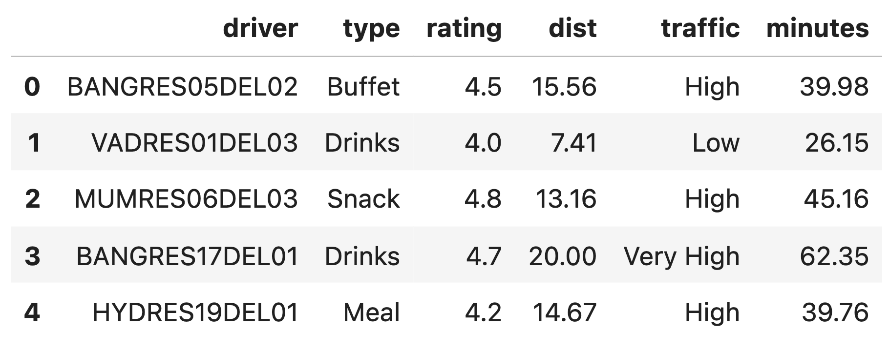
In this exam, we’ll work with the DataFrame orders,
which contains information about deliveries made using various food
delivery services in India.
The first few rows of orders are shown below, but
orders has many more rows than are shown.
Each row in orders contains information about a single
delivery. The columns in orders are as follows:
"driver" (str): The delivery driver’s ID. Note that
there are duplicate values in this column, because some drivers have
made multiple deliveries.
"type" (str): The type of food ordered; either
"Buffet", "Drinks", "Meal", or
"Snack".
"rating" (float): The average rating of the driver
out of 5, after making the given delivery.
"dist" (float): The distance from the restaurant to
the delivery address, in kilometers.
"traffic" (str): The level of traffic; either
"High", "Low", "Moderate", or
"Very High".
"minutes" (float): The time in minutes between when
a customer places their order and when they receive it.
Throughout the exam, assume we have already run all necessary import statements.
Make sure you have read the Data Overview before beginning!
Driver "WOLVAA01" has made several deliveries. Write an
expression that evaluates to the number of minutes
"WOLVAA01" took to deliver their
second-fastest order.
Answer:
orders.loc[orders["driver"] == "WOLVAA01", "minutes"].sort_values().iloc[1] or
orders.loc[orders["driver"] == "WOLVAA01", "minutes"].sort_values(ascending=False).iloc[-2]loc helps us extract a subset of the rows and columns in
a DataFrame. In general, loc works as follows:
orders.loc[<subset of rows>, <subset of columns>]Here:
We want all of the rows where orders["driver"] is
equal to "WOLVAA01", so we use the expression
orders["driver"] == "WOLVAA01" as the first input to
loc. (Remember, orders["driver"] == "WOLVAA01"
is a Series of Trues and Falses; only the
True values are kept in the result.)
We want just the column "minutes", so we supply it
as a string as the second input to loc.
Now, we have a Series with the minutes of all orders that
"WOLVAA01" has reviewed; calling the
.sort_values() method on this Series will give us back
another Series with the minutes of the orders sorted by default in
ascending order. Since we are looking for the second fastest order, we
can then use iloc to extract this value. As Python is
zero-indexed this value will be 1.
Similarly, if you specify ascending=False as a parameter
to .sort_values(), the orders will be sorted in descending
order with the order taking the longest amount of time being on top. In
such a case, we would want to extract the second last element from the
series.
Drivers’ ratings can change over time, as they perform more and more
deliveries. For instance, after one delivery a driver’s rating might be
4.8, and after their next delivery it might drop to 4.7. We say a driver
is consistent if their rating was the exact
same for all of their deliveries in orders.
Fill in the blanks so prop_consistent below evaluates to
a float, corresponding to the proportion of drivers who
are consistent.
    def f(x):
        return __(iv)__
prop_consistent = (
orders
.groupby(__(i)__)
[__(ii)__]
.__(iii)__(f)
.mean()
)Answer:
(i): "Driver". We use groupby("Driver")
because we want to check the consistency of ratings for each
individual driver. By grouping by "Driver", we are
able to look at each driver’s set of ratings across their
deliveries.
(ii): "rating". We want to check whether all
"rating" values for a given "Driver" are the
same. To do so, we’ll need to look at a Series of "rating"
values for each "Driver", so that’s the column we extract
here.
(iii): agg. The agg method allows us to
apply an aggregation function to each group (each "Driver"
in this case). This is necessary because we are checking a condition
across an entire group of ratings rather than filtering individual rows.
It’s also worth noting that since .mean() is used at the
end, the agg step must be producing a series of Boolean
values (True or False), one for each
"Driver". Each value represents whether that
driver’s ratings are consistent.
(iv): x.max() == x.min() or x.nunique() == 1. This
is the Boolean statement used in the f function to check
whether a "Driver"’s ratings are consistent.
x.max() == x.min() confirms that all ratings are identical,
since both the maximum and minimum must be the same if no variation
exists. x.nunique() == 1 achieves the same goal by checking
directly whether there is only one unique rating. Either approach is
valid, and there are several other possibilities too, such as checking
x.std() == 0 or using
x.eq(x.iloc[0]).all().
Suppose the expression below evaluates to 1.
(orders[orders["type"] == "Snack"]["driver"]
 .value_counts()
 .value_counts()
 .shape[0]
)
What can we conclude about orders?
Every driver made at least 1 "Snack" delivery.
Every driver made exactly 1 "Snack" delivery.
Every driver made at most 1 "Snack" delivery.
Every driver made exactly k
"Snack" deliveries, where k is some positive constant.
Every driver made exactly 0 or exactly k "Snack" deliveries, where
k is some positive constant.
Every driver that made a "Snack" delivery did not make
any other kind of delivery.
Answer: Every driver made exactly 0 or exactly k "Snack" deliveries, where
k is some positive constant.
The expression runs a query on the orders DataFrame,
selecting only rows where the "type" is equal to
"Snack". This narrows the focus to the set of deliveries
that were for "Snack" items. The code then selects the
"driver" column to identify which driver handled each
"Snack" delivery.
The first .value_counts() computes how many
"Snack" deliveries each "driver" made. The
second .value_counts() then counts how many drivers made
each possible number of "Snack" deliveries.
Finally, .shape[0] measures how many distinct numbers of
"Snack" deliveries were made by drivers. Since the
expression evaluates to 1, we can conclude that there is
only one distinct number of "Snack" deliveries made by
drivers. This implies that every driver either made exactly 0 or exactly
k "Snack" deliveries.
In one English sentence, describe what the following expression computes. Your sentence should start with “The driver” and should be understandable by someone who has never written code before, i.e. it should not use any technical terms.
(orders
    .groupby("Driver")
    .filter(lambda df: df.shape[0] >= 10 and df["rating"].min() >= 4.5)
    .groupby("Driver")
    ["minutes"]
    .sum()
    .idxmax()
)Answer: The driver who has driven the most minutes
total, among all "Driver"s with at least 10 deliveries and
a minimum review rating of 4.5.
The expression first groups the data by the "Driver"
column. It then filters the groups to only include those where the
"Driver" has made at least 10 deliveries and has a minimum
"rating" of 4.5. Only "Driver"s who meet both
conditions are kept in the output.
After filtering, the data is grouped by "Driver" again,
and the total number of "minutes" each
"Driver" has driven is calculated. Finally,
.idxmax() identifies the "Driver" who has
driven the most "minutes" among all "Driver"s
that fit the two criteria above.
Consider the DataFrame C, defined below.
C = orders.pivot_table(
  index="type",  # Possible values: "Buffet", "Drinks", "Meal", "Snack"
  columns="traffic",  # Possible values: "High", "Low", "Moderate", "Very Low"
  values="minutes",
  aggfunc="count"
)
Throughout this question, assume that after defining C
above, we sort C such that both its index and
columns are in ascending alphabetical order (as shown
above).
Fill in the blanks so that the expression below evaluates to the
proportion of "Snack" deliveries that were made in
"Moderate" traffic. Each blank should be filled
with a single integer, float, string, or Boolean value.
C.iloc[__(i)__, __(ii)__] / C.loc[__(iii)__].sum()Answer: There are multiple possible answers.
(i): 3 or -1. The index of C is sorted
alphabetically, meaning the row order follows "Buffet",
"Drinks", "Meal", "Snack". Since
"Snack" is the last item in this order, its index is 3
(0-based) or -1 (negative indexing).
(ii): 2 or -2. Similarly, the columns are sorted
alphabetically: "High", "Low",
"Moderate", "Very Low".
"Moderate" appears third in this order, making its index 2
(0-based) or -2 (negative indexing).
(iii): "Snack". To get the total number of
"Snack" deliveries across all traffic levels, we use
C.loc["Snack"]. The .sum() function then adds
up all values in that row.
Fill in the blanks so that the expression below evaluates to the
proportion of deliveries made in "Low" traffic that
were for "Buffet". Blanks (i) and (ii) should each
be filled with a single integer, float, string, or Boolean value.
C.loc[__(i)__, __(ii)__] / __(iii)__.sum()Options for (iii):
C.iloc[:, -1]
C.iloc[:, 0]
C.iloc[:, 1]
C.iloc[-1, :]
C.iloc[0, :]
C.iloc[1, :]
Answer: - (i): "Buffet". When using
.loc, we reference labels instead of numerical indices.
Since the index represents order "type" and is sorted
alphabetically ("Buffet", "Drinks",
"Meal", "Snack"), "Buffet" is the
correct label for selecting the row corresponding to buffet orders.
(ii): "Low". Similarly, the column order is sorted
alphabetically as "High", "Low",
"Moderate", "Very Low", making
"Low" the correct column label to select deliveries in
"Low" traffic.
(iii): C.iloc[:, 1]. Here, we are using
.iloc, which is integer-location based indexing. The
[:, 1] part means we are selecting all rows
(:) in the second column (index 1), which corresponds to
"Low" traffic, since the columns are sorted alphabetically.
By selecting C.iloc[:, 1], we are referencing all the
values in the "Low" column, and .sum() will
give the total number of deliveries made in "Low" traffic
across all order types.
Consider the DataFrames A and B, shown
below in their entirety.
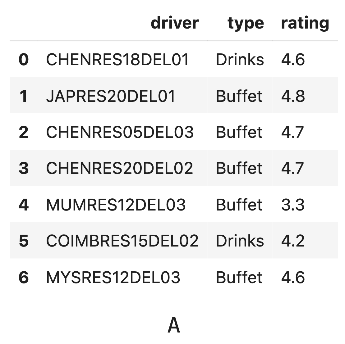
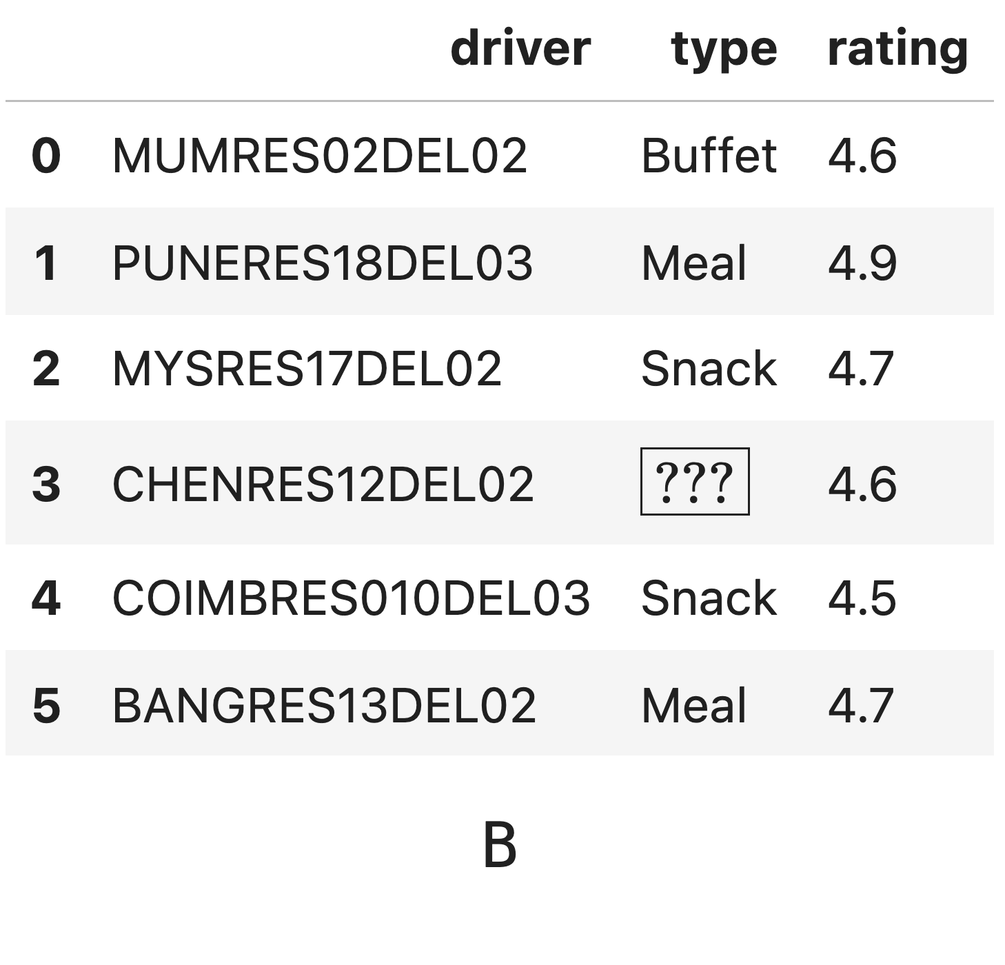
Note that the "type" value in row 3 of
DataFrame B is unknown.
Remember from the Data Overview page that the only possible values in
the "type" column are "Buffet",
"Drinks", "Meal", and
"Snack".
Suppose the DataFrame A.merge(B, on="type") has 7
rows.
What must the unknown value, \boxed{\text{???}}, be?
"Drinks"
"Buffet"
"Meal"
"Snack"
Answer: "Drinks"
Given that the resulting DataFrame after the merge has 7 rows, this
means that there are 7 matches between the rows in A and B based on the
"type" column. The value in the third row of DataFrame B is
unknown. We need to figure out which value for "type" will
give exactly 7 matches when merged with A.
Since merging on "type" generates rows where both
DataFrames have the same "type", we need to look at the
counts of each type in A and B to deduce which value the unknown
"type" should be. We can see that there are 5 rows with
type "Buffet" in DataFrame A and 1 row with type
"Buffet" in DataFrame B. This means in our merged dataset
we will have at least 5 rows of "Buffet".
We can then go through each of the different options to see which option will give us exactly 7 rows in our merged dataset. If the unknown value is:
Drinks: We have 2 rows with type
"Drinks" in DataFrame A and 1 row with type
"Drinks" (unknown value replaced) in DataFrame B, which
gives us 2 \times 1 = 2 rows in our
merged dataset. This is the correct answer because now we will have 5
(Buffet rows) + 2 (Drinks rows) = 7 rows in the merged dataset.
Buffet: We have 5 rows of "Buffet"
in DataFrame A and 2 rows in DataFrame B, which gives us 2 \times 5 = 10 rows in our merged
dataset.
Meal: We have 0 rows of "Meal" in
DataFrame A and 2 row in DataFrame B, which gives us 0 \times 2 = 0 row in our merged
dataset.
Snack: We have 0 rows of "Snack" in
DataFrame A and 3 rows in DataFrame B, which gives us 0 \times 3 = 0 rows in our merged dataset.
This is the correct answer because now we will have exactly 10 rows (all
Buffet rows) in total.
Suppose the DataFrame A.merge(B, on="type") has 10
rows.
What must the unknown value, \boxed{\text{???}}, be?
"Drinks"
"Buffet"
"Meal"
"Snack"
Answer: "Buffet"
Using the same logic as in the solution to 6.1, if the unknown value
is "Buffet", the merged dataset will include:
5 (Buffet rows from A) * 2
(Buffet rows from B) = 10 rows.This matches the stated total, so the unknown must be
"Buffet".
Suppose the DataFrame A.merge(B, on="type", how="outer")
has k rows.
The value of k depends on the unknown
value, \boxed{\text{???}}.
Which integer below cannot be k?
11
12
14
16
Answer: 14
We can replace the unknown value with each type and compute how many rows we expect to see in the final dataset after an outer merge:
Thus, the only possible number of rows that cannot occur is 14.
Suppose the unknown value, \boxed{\text{???}}, is
"Buffet".
How many rows are in the DataFrame
A.merge(B, on=["type", "rating"])?
0
1
2
3
4
5
6
7
Answer: 2
When merging on both "type" and "rating",
only exact matches in both columns will contribute to the result. Since
the unknown value is "Buffet", the only matching
combination is "Buffet" with rating 4.6, which
appears once in each DataFrame.
Thus, the total number of rows is
1 (from A) * 1 (from B) = 1 per matching pair, and if both
datasets hold one each, the result has 2 rows.
The delivery company wants to reward a subset of its drivers with a gift card for their service. To do so, they:
Choose an integer k between 1 and 10 inclusive, uniformly at random.
Choose k unique drivers, uniformly at random, such that all drivers have the same chance of being chosen, no matter how many deliveries they have made. Note that a driver cannot be selected more than once.
Driver "WOLVAA01" asks ChatGPT to write code that
simulates the probability that he wins a gift card, and it gives him
back the following:
    drivers = orders["driver"].unique()

    def choose_k():
        return np.random.choice(np.arange(1, 11))

    def one_sim(k):
        selected = np.array([])
        for i in range(k):
            selectee = np.random.choice(drivers, 1, replace=False)
            selected = np.append(selected, selectee)
        return "WOLVAA01" in selected

    def simulation():
        k = choose_k()
        N = 100_000
        total = 0
        for i in range(N):
            total = total + one_sim(k)
        return total / N
simulation() should return an estimate of the
probability that "WOLVAA01" wins a gift card, but some of
the code is potentially buggy. Select all issues with
the code above.
drivers only includes the drivers that made one
delivery, rather than all drivers.
choose_k returns a random integer between 1
and 11, instead of one from 1 to
10.
choose_k always returns the same number.
one_sim draws k drivers with replacement,
instead of without replacement.
one_sim draws k drivers without
replacement, instead of with replacement.
one_sim always returns False, because
selected is always an empty array.
simulation only picks one value of k, when
it should select a new k on each iteration.
None of the above.
Correct answers:
one_sim draws k drivers with replacement,
instead of without replacementsimulation only picks one value of k, when
it should select a new k on each iterationone_sim draws k drivers with
replacement, instead of without replacement
Because np.random.choice() is called separately each
time within the for loop, there is no guarantee that all k chosen
drivers will be distinct across iterations. Which means that some
drivers might be picked more than once, violating the “unique drivers”
requirement. The correct way to choose the k drivers would be -
np.random.choice(drivers, k, replace=False)simulation only picks one value of
k, when it should select a new k on each
iteration
The code defines k once at the beginning of simulation() using
choose_k(). This means that the same value of k is used for
all iterations of the simulation. However, as per the problem statement,
k should be chosen anew on each iteration of the simulation. Therefore,
the function choose_k() should be called within the loop to
select a random k for each iteration.
Now, for the other options:
drivers only includes the drivers that made
one delivery, rather than all drivers
orders["driver"].unique() returns all unique drivers,
regardless of how many deliveries they made, so this issue doesn’t exist
in the code.
choose_k returns a random integer between
1 and 11, instead of one from 1
to 10
np.random.choice(np.arange(1, 11)) correctly selects a
random integer from 1 to 10 (inclusive), so this is not an
issue.
choose_k always returns the same
number
choose_k() generates a random number between 1 and 10
every time it is called. Therefore, it does not always return the same
number.
one_sim always returns False,
because selected is always an empty array
The array selected is updated correctly inside the loop,
and it will contain the selected drivers for the simulation, so it
doesn’t always return False.
one_sim draws k drivers without
replacement, instead of with replacement
The issue is not about drawing without replacement; the issue is that the function draws with replacement within the for loop, which could result in the same driver being chosen more than once.
Suppose the DataFrame D contains a subset of the rows in
orders, such that:
Some of the values in the "minutes" column are
missing.
None of the values in the "minutes" column are
missing for orders made in "Moderate" traffic.
Each part of this question is independent of all other parts. In each part, select all expressions that are guaranteed to evaluate to the same value, before and after the imputation code is run. The first part is done for you.
    t = lambda x: x.fillna(x.mean())
D["minutes"] = t(D["minutes"])Answer: D.shape[0]
D.shape[0] is guaranteed to evaluate to the same value
before and after the imputation code is run because it represents the
total number of rows in the DataFrame, which is unaffected by filling in
missing values. The imputation modifies the “minutes” column but does
not alter the number of rows.
 t = lambda x: x.fillna(x.mean())
 D["minutes"] = t(D["minutes"])
D["minutes"].mean()
D.loc[D["traffic"] == "Moderate", "minutes"].mean()
D.groupby("traffic")["minutes"].mean()
None of the above.
Answer: D["minutes"].mean(),
D.loc[D["traffic"] == "Moderate", "minutes"].mean()
In this imputation code we are performing mean imputation by filling the missing values with the mean of the whole dataset.
D["minutes"].mean() - As we’ve seen in class, replacing
missing values with the mean of the observed values does not change the
mean.
D.loc[D["traffic"] == "Moderate", "minutes"].mean() -
Since the imputation does not affect the rows where “traffic” is
“Moderate” (i.e., these rows already have no missing values), the mean
for this subset of the data will remain unchanged as well.
D.groupby("traffic")["minutes"].mean() - This expression
will change after imputation. The grouped means for traffic categories
that had missing values will be affected by the imputation, as we’re
replacing missing values with the overall mean rather than
group-specific means.
 t = lambda x: x.fillna(x.mean())
 D["minutes"] = D.groupby("traffic")["minutes"].transform(t)
D["minutes"].mean()
D.loc[D["traffic"] == "Moderate", "minutes"].mean()
D.groupby("traffic")["minutes"].mean()
None of the above.
Answer:
D.loc[D["traffic"] == "Moderate", "minutes"].mean(),
D.groupby("traffic")["minutes"].mean()
In this imputation code we are performing conditional mean imputation by filling the missing values with the minutes of each group of traffic.
D["minutes"].mean() - This expression will change after
imputation. When we fill missing values with group-specific means, the
overall mean can change.
D.loc[D["traffic"] == "Moderate", "minutes"].mean() -
Since the imputation only fills in missing values for the “minutes”
column based on the mean of the “minutes” values within each traffic
group, the mean for “Moderate” traffic will remain unchanged.
D.groupby("traffic")["minutes"].mean() - The imputation
groups by the “traffic” column and fills missing values using the mean
of “minutes” within each group. Since “Moderate” traffic already had no
missing values, the mean for this group will not be affected, and
neither will the means for other groups, assuming the missing values are
only filled within their respective groups.
 present = D.loc[D["minutes"].notna(), "minutes"]
 n = D["minutes"].isna().sum()
 D.loc[D["minutes"].isna(), "minutes"] = np.random.choice(present, n)
D["minutes"].mean()
D.loc[D["traffic"] == "Moderate", "minutes"].mean()
D.groupby("traffic")["minutes"].mean()
None of the above.
Answer:
D.loc[D["traffic"] == "Moderate", "minutes"].mean()
In this imputation code we are performing unconditional probabilistic imputation by filling the missing values by randomly sampling from the present values in the “minutes” column.
D["minutes"].mean() - This expression will likely change
after imputation, as we’re replacing missing values with randomly
selected observed values.
D.loc[D["traffic"] == "Moderate", "minutes"].mean() -
Since “Moderate” traffic rows have no missing values, the imputation
does not affect them. Therefore, the mean for this subset of data will
remain unchanged.
D.groupby("traffic")["minutes"].mean() - The means for
traffic categories that had missing values will likely change after
imputation, as we’re filling in those missing values with randomly
selected values from the entire dataset rather than values specific to
each traffic category.
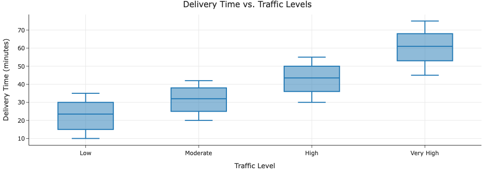
In the DataFrame orders, assume that:
The median delivery time in "Low" traffic was 22
minutes.
The median delivery time in "Moderate" traffic was
31 minutes.
The median delivery time in "High" traffic was 42
minutes.
The median delivery time in "Very High" traffic was
60 minutes.
Draw the following visualization, given the information you have.
orders.plot(kind="box", x="traffic", y="minutes")While it’s not possible to draw the visualization exactly, since you don’t have all of the exact delivery times, it is possible to roughly sketch it, such that the information provided above is clearly visible. Some additional instructions:
For simplicity, assume that across "traffic"
categories, the variation in delivery times is roughly the
same.
Make sure your axes are labeled correctly. (Hint: The y-axis should have numerical labels.)
Answer:
Consider the following corpus of two documents:
butter chicken \underbrace{\text{naan naan ... naan}}_{k \text{\: ``naan"s total}}
curry with naan
The total number of occurrences of “naan" in document 1 is k, so the total number of terms in document 1 is k + 2, where k \geq 3 is some positive integer. Note that the two documents above are the only two documents in the corpus, meaning that there are 5 unique terms total in the corpus.
Given that the cosine similarity between the bag-of-words vector representations of the two documents is \displaystyle \frac{5}{9}, what is the value of k?
3
4
5
6
7
8
9
10
Answer: 5
The bag of words vector for Document 1 is: \begin{bmatrix} 1 \\ 1 \\ k \\ 0 \\ 0 \end{bmatrix}
The bag of words vector for Document 2 is:\begin{bmatrix} 0 \\ 0 \\ 1 \\ 1 \\ 1 \end{bmatrix}
The cosine similarity can be calculated using the formula: \text{cosine sim}(\vec d_1, \vec d_2) = \frac{\vec d_1 \cdot \vec d_2}{\lVert d_1 \rVert \lVert d_2 \rVert}
For the two vectors \vec{d_1} = (1, 1, k, 0, 0) and \vec{d_2} = (0, 0, 1, 1, 1), the dot product is: \text{Dot product} = (1)(0) + (1)(0) + (k)(1) + (0)(1) + (0)(1) = k
Next, we need to calculate the magnitudes (or norms) of the two vectors. \|\vec{d_1}\| = \sqrt{1^2 + 1^2 + k^2 + 0^2 + 0^2} = \sqrt{2 + k^2}
\|\vec{d_2}\| = \sqrt{0^2 + 0^2 + 1^2 + 1^2 + 1^2} = \sqrt{3}
Substitute the values we calculated: \text{Cosine similarity} = \frac{k}{\sqrt{2 + k^2} \cdot \sqrt{3}}
We are given that the cosine similarity is \frac{5}{9}. So, we set up the equation: \frac{k}{\sqrt{2 + k^2} \cdot \sqrt{3}} = \frac{5}{9}
Solving for k gives us 5.
In this part, assume we are using a base-2 logarithm.
butter
chicken
naan
curry
with
butter
chicken
naan
curry
with
Answer:
butter and chicken
curry and with
The TF-IDF score of a term in a document is given by: \text{tf-idf}(t,d) = \text{tf}(t,d) \cdot \text{idf}(t) = \frac{\# \text{ of occurrences of } t \text{ in } d }{\text{total } \# \text{ of terms in } d} \cdot \log_2\left(\frac{\text{total } \# \text{ of documents}}{\# \text{ of documents in which } t \text{ appears}}\right)
TF-IDF scores are high when:
A term occurs frequently in the document (high TF), and
A term appears in few documents in the corpus (high IDF).
Naan appears in both documents, so its IDF is 0 and its TF-IDF is 0 in both.
Butter and chicken each appear only once, and only in document 1. So their TF is low, but their IDF is high.
Curry and with each appear only once, and only in document 2. So they also have high IDF and non-zero TF.
Therefore, butter and chicken have the highest TF-IDF in document 1, and curry and with in document 2.
This part is independent of the previous parts.
In practice, you’ll encounter lots of new metrics and formulas that you need to make sense of on the job. For instance, the Wolverine Score (WS), defined below, is an alternative to the TF-IDF that also tries to quantify the importance of a term t to a document d, given a corpus of documents d_1, d_2, ..., d_n.
\text{WS}(t, d) = \left( \frac{\text{total \# of terms in } d}{\text{\# of occurrences of } t \text{ in } d} \right) \cdot \left( \frac{\sum_{i=1}^n \text{\# of occurrences of } t \text{ in } d_i}{\sum_{i=1}^n \text{total \# of terms in } d_i} \right)
Fill in the blank to complete the statement below.
“If ___, then term t is
more common in document d than it is
across the entire corpus, and so t is
likely an important term in d."
What goes in the blank?
\text{WS}(t, d) < 0
\text{WS}(t, d) > 0
\text{WS}(t, d) < 1
\text{WS}(t, d) > 1
\text{WS}(t, d) < \frac{1}{n}, where n is the number of documents in the corpus
\text{WS}(t, d) > \frac{1}{n}, where n is the number of documents in the corpus
Answer: \text{WS}(t, d) < 1
The Wolverine Score compares a term’s relative frequency in document d versus its average frequency in the entire corpus.
The first part of WS, \frac{\text{total terms in } d}{\# \text{ of occurrences of } t \text{ in } d}, is the inverse of how frequent t is in d.
The second part, \frac{\text{total occurrences of } t \text{ in corpus}}{\text{total terms in corpus}}, is the overall frequency of t.
If WS is less than 1, it means that the term occurs more often within d than on average across all documents. This implies that the term is especially important or relevant to d.
Example: If a term appears 5 times in a 10-word document (50%), but only 10 times in a 100-word corpus (10%), then: \text{WS} = \left(\frac{10}{5}\right) \cdot \left(\frac{10}{100}\right) = 2 \cdot 0.1 = 0.2 < 1 So WS < 1 means the term is concentrated in d.
The HTML document below contains the items on Wolverine Flavors
Express’ menu. We’ve only shown three menu items, but there are many
more, as indicated by the ellipses ...
<html>
    <head>
        <title>Wolverine Flavors Express: A2's Favorite Indian Spot</title>
    </head>
    <body>
        <h1>Wolverine Flavors Express Menu</h1>
        <div class="meta">Last Updated February 25, 2025</div>
        <div class="menu-item" data-price="14.99" data-calories="650">
            <h2>Butter Chicken</h2>
            <p>Tender chicken in creamy tomato sauce - $14.99</p>
        </div>
        <div class="menu-item" data-price="12.99" data-calories="480">
            <h2>Chana Masala</h2>
            <p>Spiced chickpea curry - $12.99 ($11.99 on Tuesday)</p>
        </div>
        ...
        <div class="menu-item" data-price="21.99" data-calories="1050">
            <h2>Chicken 65 Biryani</h2>
            <p>Spicy chicken marinated with rice - $21.99 (special)</p>
        </div>
    </body>
</html>
Suppose we define soup to be a BeautifulSoup object that
is instantiated using the HTML document above. Fill in the blanks below
so that low_cals contains the names of the menu items with
less than 500 calories.
    low_cals = []
    for x in __(i)__:
        if __(ii)__:
low_cals.append(__(iii)__)Answer:
soup.find_all("div", class_="menu-item") or soup.find_all("div", attrs={"class": "menu-item"}). float(x.get("data-calories")) < 500x.find("h2").text soup.find_all("div", class_="menu-item") or soup.find_all("div", attrs={"class": "menu-item"}). We want to extract all the menu items from the HTML. Each menu item
is contained within a div tag with the class menu-item. So, we need to
find all the div elements that have this class. In BeautifulSoup, we can
do this with the find_all() method, which searches the
document for all elements matching a specific condition.
float(x.get("data-calories")) < 500 This code is used to check whether the number of calories in each
menu item is less than 500. We first use
x.get("data-calories") to retrieve the calorie count as a
string. We then convert that string to a floating-point number using
float() so we can compare it with 500. If the calorie count is less than
500, we extract the name of the menu item from the
<h2> tag and add it to the low_cals list.
x.find("h2").textLastly, we want to extract the name of the menu item from each
selected div element. The find(“h2”) method is called on x.
.find searches for the first occurrence of a
<h2> tag within the x element. Once we have the
<h2> element (in this case,
Chana Masala), we use .text to extract the text content
inside the <h2> tag.
When we originally downloaded the orders dataset from
the internet, some of the values in the "minutes" columns
were formatted incorrectly as strings with two decimals in them. To
clean the data, we implemented the function clean_minutes,
which takes in an invalid minutes value as a string and returns a
correctly formatted minutes value as a float. Example behavior of
clean_minutes is given below.
>>> clean_minutes("8.334.108")
83.34
>>> clean_minutes("5.123.999")
51.23
>>> clean_minutes("12.091.552")
120.91
>>> clean_minutes("525.345.262")
5253.45
As a helper function, we implemented the function
split_pieces; example behavior is given below.
>>> split_pieces("8.334.108")
("8", "334")
>>> split_pieces("12.091.552")
("12", "091")
Fill in the blanks to complete the implementations of the functions
split_pieces and clean_minutes so that they
behave as described above. Assume that the inputs to both functions are
formatted like in the examples above, i.e. that there are exactly 3
digits between the middle two decimals.
def split_pieces(s):
    return re.findall(__(i)__, s)[0]

def clean_minutes(s):
    p = split_pieces(s)
return __(ii)__Answer:
(\d+)\.(\d{3})
int(p[0] + p[1]) / 100
(\d+)\.(\d{3})
(\d+): This part matches one or more digits before the
first decimal point. The parentheses around capture this part into a
group, allowing us to extract the digits before the first decimal.
\.: This matches the literal decimal point. The
backslash is necessary because the dot . is a special character in
regular expressions that usually matches any character, so we need to
escape it with a backslash to match an actual period.
(\d{3}): This matches exactly three digits after the
first decimal and before the second decimal. The parentheses around
capture these digits into another group, allowing us to extract them
separately.
int(p[0] + p[1]) / 100 p is a tuple returned by the split_pieces(s) function, where p[0] is the first part (before the first decimal point) and p[1] is the part between the two decimals.
For example, if the input string is “8.334.108”, p would be (“8”,
“334”). The expression python p[0] + p[1] concatenates
these two parts together, creating the string “83334”. This represents
the combined value of the minutes, but it’s not in the correct format.
We can wrap this around the int function which will convert the
concatenated string “83334” into an integer.
Suppose we’d like to fit a constant model, H(x_i) = h, to predict the number of minutes a delivery will take. To find the optimal constant prediction, h^*, we decide to use the \alpha \beta-balanced loss function, defined below:
L_{\alpha \beta}(y_i, h) = (\alpha y_i - \beta h)^2
where \alpha and \beta are both constants, and \beta \neq 0.
Below, assume \bar{y} = \frac{1}{n} \sum_{i = 1}^n y_i is the mean number of minutes a delivery took.
Suppose \alpha = 3 and \beta = 3, so L_{\alpha \beta}(y_i, h) = (3y_i - 3h)^2.
What is the optimal constant prediction, h^*, that minimizes average \alpha \beta-balanced loss?
\bar{y}
\frac{1}{2} \bar{y}
2 \bar{y}
\frac{1}{3} \bar{y}
3 \bar{y}
\frac{1}{6} \bar{y}
6 \bar{y}
Answer: \bar{y}
To find the optimal parameter, we have to minimize the average loss function. The loss function is given as: L_{\alpha \beta}(y_i, h) = (3y_i - 3h)^2
To minimize this, we need to find the value of h that minimizes the sum of squared errors for all y_{i}. We do this by taking the derivative of the loss function and solving it by setting it to zero.
Expanding the squared term: \sum_{i=1}^{n} (9y_i^2 - 18y_i h + 9h^2)
Using summation properties: 9 \sum_{i=1}^{n} y_i^2 - 18h \sum_{i=1}^{n} y_i + 9h^2 n
Differentiating: \frac{d}{dh} \left( 9 \sum_{i=1}^{n} y_i^2 - 18h \sum_{i=1}^{n} y_i + 9h^2 n \right)
Since the first term 9 \sum_{i=1}^{n} y_i^2 does not depend on h, its derivative is zero.
Differentiating the remaining terms: \frac{d}{dh} (-18h \sum_{i=1}^{n} y_i) = -18 \sum_{i=1}^{n} y_i
\frac{d}{dh} (9h^2 n) = 18h n
Thus, the derivative of the total loss is: -18 \sum_{i=1}^{n} y_i + 18h n
Setting the derivative equal to zero: -18 \sum_{i=1}^{n} y_i + 18h n = 0
Dividing both sides by 18: - \sum_{i=1}^{n} y_i + h n = 0
Solving for h: h = \frac{\sum_{i=1}^{n} y_i}{n}
This is equivalent to mean of \bar{y}. Thus, the optimal constant prediction is the mean of the delivery times.
Suppose \alpha = 6 and \beta = 3, so L_{\alpha \beta}(y_i, h) = (6y_i - 3h)^2.
What is the optimal constant prediction, h^*, that minimizes average \alpha \beta-balanced loss?
\bar{y}
\frac{1}{2} \bar{y}
2 \bar{y}
\frac{1}{3} \bar{y}
3 \bar{y}
\frac{1}{6} \bar{y}
6 \bar{y}
Answer: 2 \bar{y}
To find the optimal parameter, we have to minimize the average loss
function. The loss function is given as:
L_{\alpha \beta}(y_i, h) = (6y_i -
3h)^2
To minimize this, we need to find the value of h that minimizes the sum of squared errors for all y_i. We do this by taking the derivative of the loss function and solving it by setting it to zero.
Expanding the squared term: \sum_{i=1}^{n} (36y_i^2 - 36y_i h + 9h^2)
Using summation properties: 36 \sum_{i=1}^{n} y_i^2 - 36h \sum_{i=1}^{n} y_i + 9h^2 n
Differentiating: \frac{d}{dh} \left( 36 \sum_{i=1}^{n} y_i^2 - 36h \sum_{i=1}^{n} y_i + 9h^2 n \right)
Since the first term 36 \sum_{i=1}^{n} y_i^2 does not depend on h, its derivative is zero.
Differentiating the remaining terms: \frac{d}{dh} (-36h \sum_{i=1}^{n} y_i) = -36 \sum_{i=1}^{n} y_i
\frac{d}{dh} (9h^2 n) = 18h n
Thus, the derivative of the total loss is: -36 \sum_{i=1}^{n} y_i + 18h n
Setting the derivative equal to zero: -36 \sum_{i=1}^{n} y_i + 18h n = 0
Dividing both sides by 18: -2 \sum_{i=1}^{n} y_i + h n = 0
Solving for h: h = \frac{2 \sum_{i=1}^{n} y_i}{n} = 2 \bar{y}
Thus, the optimal constant prediction is 2 \bar{y}.
Find the optimal constant prediction, h^*, that minimizes average \alpha \beta-balanced loss in general, for any valid choice of \alpha and \beta. Show your work, and \boxed{\text{box}} your final answer, which should be an expression involving \bar{y}, \alpha, \beta, and/or other constants.
Answer: \frac{\alpha}{\beta} \bar{y}
To find the optimal parameter, we have to minimize the average loss
function. The loss function is given as:
L_{\alpha \beta}(y_i, h) = (\alpha y_i -
\beta h)^2
To minimize this, we need to find the value of h that minimizes the sum of squared errors for all y_i. We do this by taking the derivative of the loss function and solving it by setting it to zero.
Expanding the squared term: \sum_{i=1}^{n} (\alpha^2 y_i^2 - 2\alpha\beta y_i h + \beta^2 h^2)
Using summation properties: \alpha^2 \sum_{i=1}^{n} y_i^2 - 2\alpha\beta h \sum_{i=1}^{n} y_i + \beta^2 h^2 n
Differentiating: \frac{d}{dh} \left( \alpha^2 \sum_{i=1}^{n} y_i^2 - 2\alpha\beta h \sum_{i=1}^{n} y_i + \beta^2 h^2 n \right)
Since the first term \alpha^2 \sum_{i=1}^{n} y_i^2 does not depend on h, its derivative is zero.
Differentiating the remaining terms: \frac{d}{dh} (-2\alpha\beta h \sum_{i=1}^{n} y_i) = -2\alpha\beta \sum_{i=1}^{n} y_i
\frac{d}{dh} (\beta^2 h^2 n) = 2\beta^2 h n
Thus, the derivative of the total loss is: -2\alpha\beta \sum_{i=1}^{n} y_i + 2\beta^2 h n
Setting the derivative equal to zero: -2\alpha\beta \sum_{i=1}^{n} y_i + 2\beta^2 h n = 0
Dividing both sides by 2: - \alpha\beta \sum_{i=1}^{n} y_i + \beta^2 h n = 0
Solving for h: h = \frac{\alpha\beta \sum_{i=1}^{n} y_i}{\beta^2 n}
We substitute \sum_{i=1}^{n} y_i = n\bar{y} into the equation: h = \frac{\alpha\beta (n\bar{y})}{\beta^2 n}
This simplified gives us h^* = \frac{\alpha}{\beta} \bar{y}
Suppose we’d like to predict the number of minutes a delivery will take (y) as a function of distance (x). To do so, we look to our dataset of n deliveries, (x_1, y_1), (x_2, y_2), ..., (x_n, y_n), and fit two simple linear models:
F(x_i) = a_0 + a_1 x_i, where: a_1 = r \frac{\sigma_y}{\sigma_x}, \qquad a_0 = \bar{y} - r \frac{\sigma_y}{\sigma_x} \bar{x}
Here, r is the correlation coefficient between x and y, \bar{x} and \bar{y} are the means of x and y, respectively, and \sigma_x and \sigma_y are the standard deviations of x and y, respectively.
G(x_i) = b_0 + b_1 x_i, where b_0 and b_1 are chosen such that the line G(x_i) = b_0 + b_1 x_i minimizes mean absolute error on the dataset. Assume that no other line minimizes mean absolute error on the dataset, i.e. that the values of b_0 and b_1 are unique.
Fill in the \boxed{\text{???}}: \displaystyle \sum_{i = 1}^n (y_i - G(x_i))^2 \:\:\: \boxed{???} \:\:\: \sum_{i = 1}^n (y_i - F(x_i))^2
\geq
>
=
<
\leq
Impossible to tell
Answer: >
The quantity \frac{1}{n} \sum_{i = 1}^n (y_i - F(x_i))^2 is the mean squared error (MSE) of model F. By definition, F is the line that minimizes MSE over all possible linear models.
The quantity \frac{1}{n} \sum_{i = 1}^n (y_i - G(x_i))^2 is the mean squared error of model G, which is not optimized for MSE but rather for mean absolute error (MAE).
Since F is specifically constructed
to minimize the squared error, and G is
not, we must have:
\sum_{i = 1}^{n} (y_i - G(x_i))^2 >
\sum_{i = 1}^{n} (y_i - F(x_i))^2
Fill in the \boxed{\text{???}}: \displaystyle \left( \sum_{i = 1}^n \big| y_i - G(x_i) \big| \right)^2 \:\:\: \boxed{???} \:\:\: \left( \sum_{i = 1}^n \big| y_i - F(x_i) \big| \right)^2
\geq
>
=
<
\leq
Impossible to tell
Answer: <
The quantity \frac{1}{n} \sum_{i = 1}^n | y_i - G(x_i) | is the mean absolute error (MAE) of model G. By definition, G is the line that minimizes MAE over all possible linear models.
The quantity \frac{1}{n} \sum_{i = 1}^n | y_i - F(x_i) | is the mean absolute error of model F, which is not optimized for MAE but rather for mean squared error (MSE).
Since G is specifically constructed
to minimize the absolute error, and F
is not, we must have:
\sum_{i = 1}^{n} | y_i - G(x_i) | <
\sum_{i = 1}^{n} | y_i - F(x_i) |
Squaring both sides preserves the inequality (since both sides are
non-negative), so:
\left( \sum_{i = 1}^{n} | y_i - G(x_i) |
\right)^2 < \left( \sum_{i = 1}^{n} | y_i - F(x_i) | \right)^2
Below, we’ve drawn both lines, F, and G, along with a scatter plot of the original n deliveries.
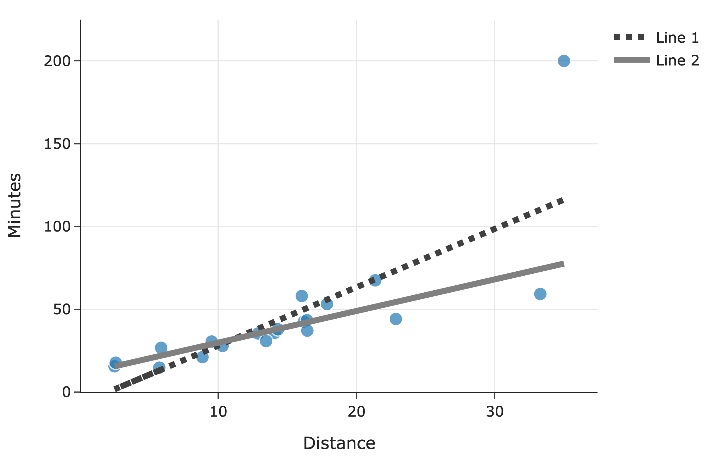
Which line corresponds to line F?
Line 1
Line 2
Answer: Line 1
The key idea is that models trained with squared loss (MSE) are more sensitive to outliers than models trained with absolute loss (MAE).
Since Line 1 appears to be “pulled up” more strongly by an outlier, it suggests that this line was influenced more heavily by extreme values. This behavior aligns with how MSE-based regression works: outliers have a greater impact on the overall loss because squaring the errors makes large deviations even more significant.
In contrast, MAE-based regression (Line 2) is less sensitive to outliers because absolute differences do not grow as quickly.
Therefore, Line 1 corresponds to F, the MSE-minimizing line.
Optional
In Question 7, assuming that there are 100 unique drivers, what is
the true, theoretical probability that "WOLVAA01" wins a
free gift card? Show your work, and your final answer, which should be a
fraction.
Don’t spend time on this question if you haven’t attempted all other
questions, as it is purely for (very little)
extra credit.
Answer: \frac{55}{100}
We have 100 unique drivers and 10 different groups. The probability
that "WOLVAA01" wins is calculated by adding up the chances
that it is chosen in each group.
For each group, the probability of winning depends on how many drivers are in that group. For example:
"WOLVAA01"
wins is \frac{1}{10} \times
\frac{1}{100}.The total probability is the sum of these individual probabilities: \text{Total Probability} = \frac{1}{10} \times \frac{1}{100} + \frac{1}{10} \times \frac{2}{100} + \cdots + \frac{1}{10} \times \frac{10}{100} which simplifies to: \text{Total Probability} = \frac{1}{1000} (1 + 2 + \cdots + 10) = \frac{1}{1000} \times 55 = \frac{55}{1000} = \frac{55}{100}.