← return to study.practicaldsc.org
Instructor(s): Suraj Rampure
This exam was administered in-person. The exam was closed-notes,
except students were allowed to bring a single two-sided notes sheet. No
calculators were allowed. Students had 120 minutes to take this exam.
Access the original exam PDF
here.
In this exam, we’ll work with the DataFrame fish, which
contains information about various fish for sale at a market in
Finland.
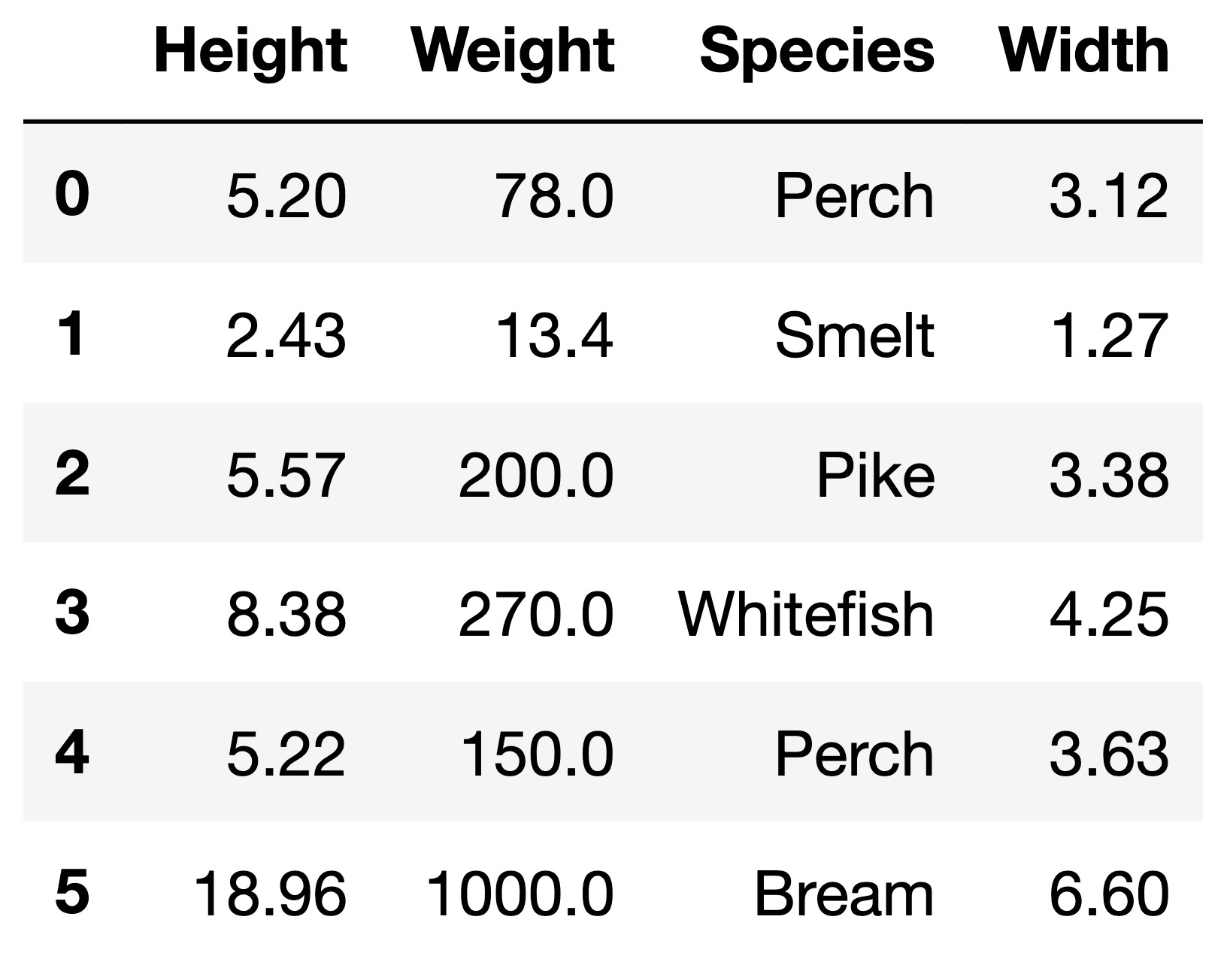
The first few rows of fish are shown below, but
fish has many more rows than are shown.
Each row in fish contains information about a single
fish. The columns in fish are as follows:
"Height" (float): The height of the fish, in
inches.
"Weight" (float): The weight of the fish, in
grams.
"Species" (str): The species of the fish. There are
7 possible species, 5 of which are shown in the example
above.
"Width" (float): The width of the fish, in
inches.
Throughout the exam, assume we have already run all necessary import statements.
Suppose we use the code below to build a multiple linear regression model to predict the width of a fish, given its height and weight.
X, _, y, _ = train_test_split(fish["Height", "Weight"], fish["Width"])
model = LinearRegression()
model.fit(X, y)

# Used in the grid below.
ws = np.append(model.intercept_, model.coef_)
preds = model.predict(X)
squares = X.shape[0] * mean_squared_error(y, preds)
Assume that:
X and \texttt{X} both represent the design matrix used to train the model, and that X is full rank.
\vec y and \texttt{y} both represent the observation vector used to train the model.
\vec w^* represents the optimal
parameter vector found by sklearn.
In each column of the grid below, select all mathematical expressions that have the same value as the code expression provided in the column header. The first column has been done for you as an example. Some guidance:
It is possible that some rows are left empty, but there should be at least one square filled in per column. Tip: Look at one column at a time.
Assume, just for this part, that \vec 0 and 0 are the same value, e.g. if an expression produces an array of 0s, you would select the 0 option in the second row.
| a) | b) | c) | d) | ||
|---|---|---|---|---|---|
X.shape[1] |
preds |
ws |
squares |
np.sum(y - preds) |
|
| 3 | ✓ | ||||
| 0 | |||||
| \lVert \vec y - X \vec w^* \rVert^2 | |||||
| X^TX \vec w^* - X^T \vec y | |||||
| \vec1^T(\vec y - X \vec w^*) | |||||
| (X^TX)^{-1}X^T \vec y | |||||
| X(X^TX)^{-1}X^T \vec y |
Answer:
| a) | b) | c) | d) | ||
|---|---|---|---|---|---|
X.shape[1] |
preds |
ws |
squares |
np.sum(y - preds) |
|
| 3 | ✓ | ||||
| 0 | ✓ | ||||
| \lVert \vec y - X \vec w^* \rVert^2 | ✓ | ||||
| X^TX \vec w^* - X^T \vec y | ✓ | ||||
| \vec1^T(\vec y - X \vec w^*) | ✓ | ||||
| (X^TX)^{-1}X^T \vec y | ✓ | ||||
| X(X^TX)^{-1}X^T \vec y | ✓ |
Suppose we’d like to build a regression model to predict the width of a fish, given its height and weight.
For each of several model instances, we train a model twice — once with the features as-is, and once with standardized features. In other words:
# Without standardization
model = ModelClass() # e.g. model = Lasso(alpha=10000)
model.fit(X, y)

# With standardization
model_std = make_pipeline(StandardScaler(), ModelClass())
model_std.fit(X, y)
We say a model is standardization invariant if its training mean squared error is guaranteed to be the same, with or without standardization. Which of the models below are standardization invariant? Select all that apply.
LinearRegression()
Ridge(alpha=10)
Lasso(alpha=1)
Lasso(alpha=10000)
DecisionTreeRegressor(max_depth=3)
KNeighborsRegressor(n_neighbors=5)
KNeighborsRegressor(n_neighbors=8)
Answer: LinearRegression() and
DecisionTreeRegressor(max_depth=3).
Let’s look at each option individually.
✅ LinearRegression(): Notice that this model
does not use regularization, i.e. the objective
function we minimize to find this model’s optimal parameter vector \vec w^* does not use regularization. As we
discussed in Lecture
16, standardizing the features of a (non-regularized) linear
regression model does not change the model’s predictions – and, hence,
does not change its training MSE – instead, it only changes its
coefficients. Hence, this model is standardization
invariant.
❌ Ridge(alpha=10): This model does
use regularization. To find this model’s optimal parameters \vec w^*, we minimize the objective function
R_\text{ridge}(\vec w) = \frac{1}{n} \lVert \vec y - X \vec w
\rVert_2^2 + \lambda \sum_{j=1}^d w_j^2
where \lambda is the regularization hyperparameter. Standardizing the model’s features changes the scales of the coefficients, which changes the size of the regularization term, \lambda \sum_{j=1}^d w_j^2. As a result, the model’s parameters will all change and its predictions will change, meaning its MSE is not guaranteed to be the same. Hence, this model is not standardization invariant.
❌ Lasso(alpha=1): Same logic as above.
❌ Lasso(alpha=10000): Same logic as
above.
✅ DecisionTreeRegressor(max_depth=3): Recall,
decision trees ask a sequence of yes/no questions using the features. If
all of the features are standardized, the questions themselves can be
rescaled in order for the tree to make the same predictions (which were
originally optimal). For example, if pre-standardization, one of the
questions was “is height < 5”, post-standardization the same question
could be “is height < -1.25”, if a height of 5 was 1.25 standard
deviations below the average height. So, this model is
standardization invariant.
❌ KNeighborsRegressor(n_neighbors=5): Recall, k-nearest neighbors classifiers make
predictions based on the distances between points. If the features are
standardized, the distances between any two points will change, which
changes the model’s predictions. Hence, this model is
not standardization invariant.
❌ KNeighborsRegressor(n_neighbors=8): Same logic as
above.
A good homework question to review here is Homework 10, Question 2.
The average score on this problem was 68%.
Consider the two model instances below.
once = make_pipeline(StandardScaler(), ModelClass())
twice = make_pipeline(StandardScaler(), StandardScaler(), ModelClass())
True or False: As long as ModelClass() is a valid
regression model in sklearn that behaves
deterministically*, once and twice are
guaranteed to have the same training mean squared
error.
True
False
By this, we mean that the model makes the same predictions every time it is fit on the same training set. Technically, not all models behave this way.
Answer: True.
Suppose x is an array containing the information for a
single feature. To standardize x, we can use the following
code:
x_std = (x - x.mean()) / x.std()x_std, by definition, has a mean of 0 and standard
deviation of 1. If we try and standardize x_std, the
resulting array will be identical to x_std. In other words,
if we run:
x_std_again = (x_std - x_std.mean()) / x_std.std()x_std.mean() is already 0, and x_std.std()
is already 1, so x_std_again is being set to
(x_std - 0) / 1, which is just x_std.
So, after we standardize a feature once, standardizing it again will not change the results.
The average score on this problem was 79%.
Suppose A \in \mathbb{R}^{n \times d} is a matrix, \vec b \in \mathbb{R}^n is a vector, \theta is a negative number, and that \vec v^* is a vector that minimizes \lVert \vec b - A \vec v \rVert^2. In other words: \vec v^* = \underset{\vec v}{\text{argmin}} \lVert \vec b - A \vec v \rVert
Furthermore, suppose that one of the columns in A is \vec \theta = \begin{bmatrix} \theta \\ \theta \\ \vdots \\ \theta\end{bmatrix}.
What is the value of \vec \theta^T (\vec b - A \vec v^*)?
0
\vec 0
1
\vec 1
\theta
\vec \theta
None of these
Note: There was originally another part of this problem, but we’ve removed it, since its answer was not well defined.
Answer: 0.
First, note that the expression \vec \theta^T (\vec b - A \vec v^*) is computing the dot product of \vec \theta and \vec b - A \vec v^*, which means the result must be a scalar. This rules \vec 0, \vec 1, and \vec \theta as possible options.
One of the big ideas in Lecture 14: Regression using Linear Algebra is that the parameter vector \vec v^* that minimizes \lVert \vec b - A \vec v \rVert^2 is chosen in order to guarantee that the columns of A are orthogonal to the error vector, \vec b - A \vec v^*. Since \vec \theta = \begin{bmatrix} \theta \\ \theta \\ \vdots \\ \theta\end{bmatrix} is a column in A, we know that \vec \theta must be orthogonal to \vec b - A \vec v^*, meaning the dot product of the two vectors in question must be 0.
The average score on this problem was 57%.
Suppose we’d like to build a regression model to predict the width of a fish, given its height, weight, and species. Consider the following two possible approaches to building linear regression models:
Approach 1: One hot encode species using
OneHotEncoder(drop="first"), use height and weight as-is,
and fit a linear regression model.
Approach 2: Fit 7 separate sub-models, one for each unique value of species, where each sub-model is a linear regression model that uses height and weight only.
For instance, one of the 7 sub-models would be for the Perch species; we’d query the training data to keep only the rows corresponding to the species Perch, then fit the Perch sub-model on just this subset of the training data.
To predict the width of a new fish, we use the sub-model corresponding to the new fish’s species.
Assume that in both approaches, the linear regression models being considered include intercept terms.
Suppose the mean squared error on the training set for approaches 1 and 2 are \text{MSE}_1 and \text{MSE}_2, respectively. Fill in the :
\displaystyle \text{MSE}_1 \:\:\: \boxed{???} \:\:\: \text{MSE}_2
\geq
>
=
<
\leq
Impossible to tell
Answer: \geq.
The key to this problem is understanding the physical difference between the two approaches.
Approach 1 one hot encodes species, meaning the model is of the form:
\text{predicted width}_i = w_0 + w_1 \cdot \text{height}_i + w_2 \cdot \text{weight}_i + w_3 \left( \text{species}_i = {\text{Perch}} \right) + w_4 \left( \text{species}_i = {\text{Smelt}} \right) + ... + w_8 \left( \text{species}_i = {\text{Bream}} \right)
Notice there are 6 species-specific parameters – this is because
there are 7 species total, and we drop one of the species to avoid
multicollinearity (through the use of drop="first" in the
OneHotEncoder).
Physically, this model looks like 7 different but parallel planes in 3D (if our axes are height, weight, and width). Each of these planes has the same slopes in the height and weight directions, but different z-intercepts.
Approach 2 fits 7 different planes in 3D, each of which has potentially different intercepts, but also potentially different slopes.
This means that Approach 2 is more flexible than Approach 1. Suppose that the way to minimize mean squared error is to create 7 parallel planes – one per species – that each have the same height and weight coefficients. Approach 1 and Approach 2 can both do that. However, Approach 2 can do more than that – it can create planes that are not parallel, and that have different height and weight coefficients for each species, and will do so if it helps minimize mean squared error further.
So, Approach 2’s mean squared error will always be less than or equal to Approach 1’s mean squared error, which means \text{MSE}_2 \leq \text{MSE}_1, or \text{MSE}_1 \boxed{\geq} \text{MSE}_2 as the question intended.
This intuition was built through Homework 7, Question 4, which introduced one hot encoding from a visual perspective.
The average score on this problem was 38%.
Suppose we visualize both models in 3 dimensions, where one axis represents height, one axis represents weight, and one axis represents predicted width.
Fill in the blanks: In the 3 dimensional space described above,
the fit model in approach 1 looks like __(i)__ __(ii)__ __(iii)__,
while the fit model in approach 2 looks like __(iv)__ __(v)__ __(vi)__.
2
3
4
5
6
7
identical
possibly non-parallel
orthogonal
parallel
lines
planes
points
spheres
vectors
2
3
4
5
6
7
identical
possibly non-parallel
orthogonal
parallel
lines
planes
points
spheres
vectors
Answer: In the 3 dimensional space described above,
the fit model in approach 1 looks like 7 parallel planes,
while the fit model in approach 2 looks like 7 possibly non-parallel planes.
The average score on this problem was 64%.
It is possible to construct a design matrix X' such that approach 2 is implemented as a single linear regression model, rather than 7 separate linear regression models.
How many columns are in the design matrix, X'?
Answer: 21.
To implement approach 2 as a single linear regression model, we need to create two slopes – one for height and one for weight – plus one intercept term, separately for each of 7 features.
To better illustrate what we mean, let’s imagine what X' might look like. For example, let’s suppose that:
Then, X' would look like:
X' = \begin{bmatrix} 1 & 50 & 25 & 0 & 0 & 0 & 0 & ... & 0\\ 0 & 0 & 0 & 1 & 2.43 & 13.4 & 0 & ... & 0 \\ \vdots & \vdots & \vdots & \vdots & \vdots & \vdots & \vdots & \vdots & \vdots \end{bmatrix}_{n \times 21}
In the example above, the first three columns are “turned on” for Perch fish only; for non-Perch fish, their values are always 0. The second set of three columns are “turned on” for Smelt fish only, and so on and so forth.
The average score on this problem was 22%.
In 1-2 English sentences, describe how to create X'. Then, sketch an example of how X' might look, including at least two example rows, one of which should correspond to a fish of the Perch species with a height of 50 and weight of 25. Feel free to use ellipses, ..., in your answer.
Answer: Answered above.
The average score on this problem was 51%.
Suppose we’d like to build a regression model to predict the width of a fish, given various features. Consider the six line graphs shown below.
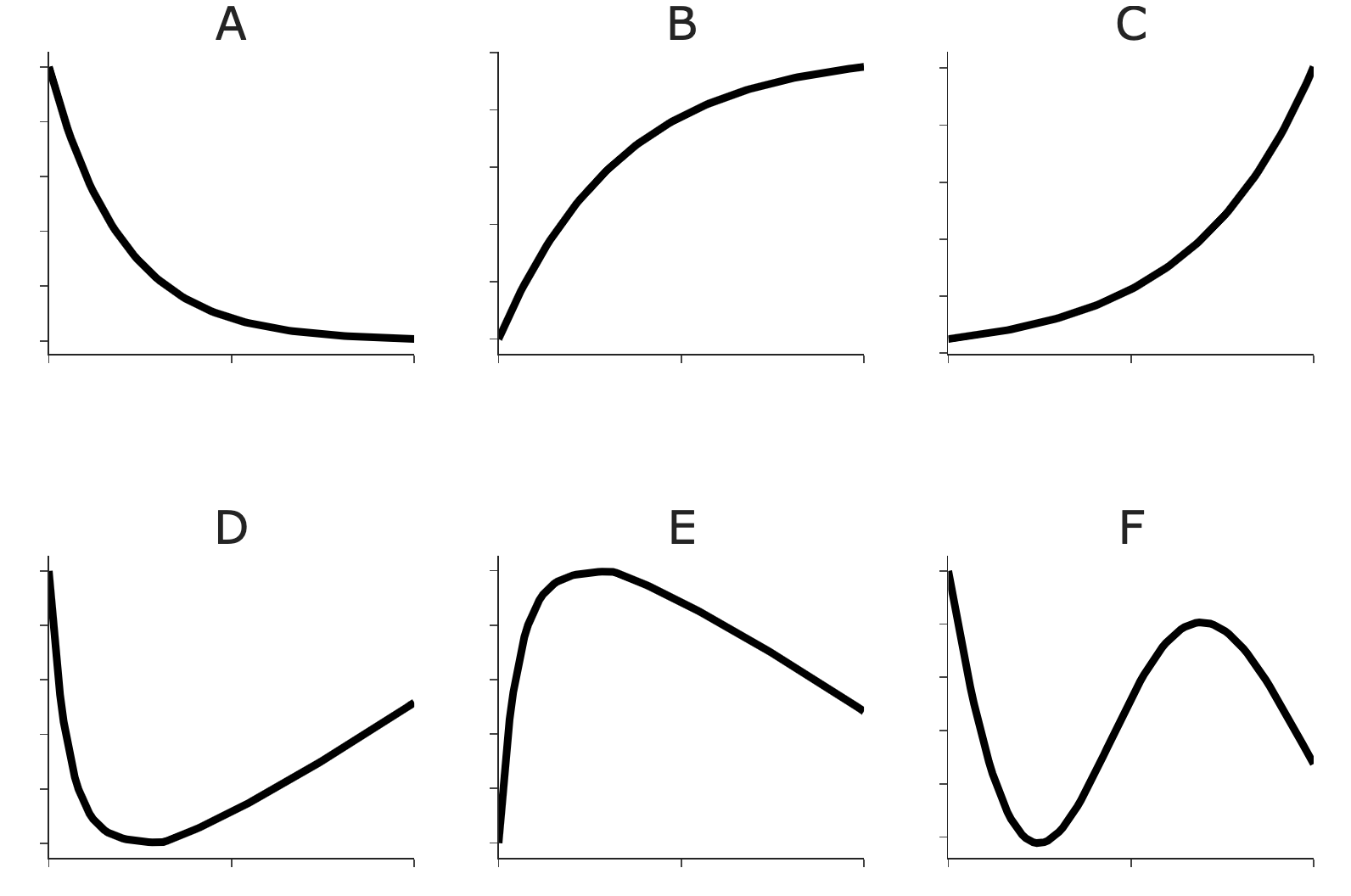
In each part, select the graph that best represents the relationship between model performance (drawn on the y-axis) and the provided hyperparameter (drawn on the x-axis).
First, suppose we build a k-nearest neighbors regression model, as seen in Homework 8.
Which graph best represents training mean squared error (y-axis) vs. k (x-axis)?
A
B
C
D
E
F
Answer: B.
Small values of k correspond to highly overfit k-nearest neighbors regression models. As we saw in Homework 8, a k-NN regression model with k=1 passes through every single training point, and has extremely low training set MSE (remember, MSE is low when model performance is “good” on the dataset we’re using for evaluation). As k increases, the model averages over more and more of the training set in order to make a prediction, and so training set MSE increases.
The average score on this problem was 100%.
Which graph best represents test set mean squared error vs. k?
A
B
C
D
E
F
Answer: D.
A common pattern we’ve seen is that as model complexity increases, test set performance improves until a “sweet spot”, and then worsens as the model starts to overfit. Here, as k increases, model complexity decreases, though the graph of test set MSE would be the same as if increasing k increases model complexity – it should decrease to a point, then increase again. This is precisely what happens in Option D.
The average score on this problem was 72%.
Which graph best represents model variance vs. k?
A
B
C
D
E
F
Answer: A.
As explained in the answer to 5.1, as k increases, model complexity decreases, and hence model variance decreases.
The average score on this problem was 48%.
Now, suppose we build a linear regression model with degree-d polynomial features.
Which graph best represents training mean squared error vs. d?
A
B
C
D
E
F
Asnwer: A.
As d increases here, model complexity increases, so the model’s tendency to overfit to training sets increases, and so training set MSE decreases.
The average score on this problem was 79%.
Which graph best represents test set R^2 vs. d? Hint: Recall from Homework 8, 0 \leq R^2 \leq 1, where larger values of R^2 indicate better predictions.
A
B
C
D
E
F
Answer: E.
As d increases – i.e. as model complexity increases – test set performance increases until a sweet spot, then decreases again once the model is too complex. The difference between R^2 and MSE is that large R^2 values correspond to better model performance, while large MSE values correspond to worse model performance. So, we’re looking for a graph that first increases and then decreases vertically, which matches Option E. (Notice that E looks like an upside-down version of D, which would be the answer if we were asked for the graph that represents test set MSE vs. d.)
The average score on this problem was 74%.
Which graph best represents model variance vs. d?
A
B
C
D
E
F
Answer: C.
As d increases, model complexity increases, so model variance increases as well. There’s no reason to believe model variance is bounded, as Option B indicates, hence Option C is the correct answer.
The average score on this problem was 64%.
Finally, suppose we build a ridge regression model with hyperparameter \lambda.
Which graph best represents model variance vs. \lambda?
A
B
C
D
E
F
Answer: A.
As \lambda increases, model complexity decreases, and hence model variance decreases.
The average score on this problem was 74%.
Suppose we’d like to build a L_1-regularized (LASSO) regression model to predict the width of a fish, given its height and weight. To choose a value of \lambda (the regularization hyperparameter) from the list [0.01, 0.1, 1, 10], we perform k-fold cross-validation with k=4.
Consider the following optimal parameter vectors, each of which came from minimizing L_1-regularized empirical risk using a different value of \lambda.
(In each parameter vector, the 0th component represents the intercept term, the 1st component represents the coefficient on height, and the 2nd component represents the coefficient on weight.)
\vec{w}_a^* = \begin{bmatrix} 2.6999 \\ 0.0105 \\ 0.0041 \end{bmatrix} \qquad \vec{w}_b^* = \begin{bmatrix} 3.0674 \\ 0.0000 \\ 0.0034 \end{bmatrix} \qquad \vec{w}_c^* = \begin{bmatrix} 2.0728 \\ 0.1236 \\ 0.0031 \end{bmatrix}
Which optimal parameter vector came from choosing \lambda = 0.01?
\vec w_a^*
\vec w_b^*
\vec w_c^*
Which optimal parameter vector came from choosing \lambda = 0.1?
\vec w_a^*
\vec w_b^*
\vec w_c^*
Which optimal parameter vector came from choosing \lambda = 1?
\vec w_a^*
\vec w_b^*
\vec w_c^*
Answer:
When performing regularization, as \lambda increases, the model’s optimal parameters (except for the intercept term!) decrease in magnitude, since we’re penalizing the sizes of the model’s parameters in the objective function:
R_\text{LASSO}(\vec w) = \frac{1}{n} \lVert \vec y - X \vec w \rVert^2 + \lambda \sum_{j=1}^d |w_i|
In the case of L_1 regularization (i.e. LASSO), as illustrated above, the model’s optimal parameters shrink towards 0 exactly, for reasons discussed in Lecture 19. As the formula above dictates, we do not penalize the intercept term, w_0.
So, since \lambda = 1 has the largest value of \lambda among the values we are considering, it corresponds to the optimal parameter vector in which the non-intercept parameters are the smallest, which is \vec w_b^*. \lambda = 0.01 has the smallest value of \lambda among the values we are considering, so it corresponds to the optimal parameter vector that seems the least regularized, i.e. in which the non-intercept parameters are the largest, which is \vec w_c^*. \lambda = 0.1, by process of elimination, corresponds to \vec w_a^*.
The average score on this problem was 79%.
Suppose, just for this part, that:
Our entire dataset has N rows.
To split the dataset of N rows
into training and test sets, we use train_test_split with
test_size=0.2.
While performing 4-fold cross-validation, each time a model is trained, 90 points are used to train the model. What is the value of N?
100
108
120
150
180
None of these
Answer: 150.
test_size=0.2, 80% of the data is
used for training, and 20% is used for testing, and so the training set
size is \frac{4}{5}N.
The average score on this problem was 44%.
Average validation mean squared errors are shown in the table below.
| Fold 1 | Fold 2 | Fold 3 | Fold 4 | |
| λ = 0.01 | 15 | 9 | 12 | 12 |
| λ = 0.1 | 12 | 18 | 6 | 12 |
| λ = 1 | 3 | 12 | 15 | m |
| λ = 10 | 18 | 6 | 3 | 9 |
Given that \lambda = 1 is the hyperparameter with the best cross-validation performance above, provide the best possible upper-bound for a value of m. That is, find M such that, as long as m < M, \lambda = 1 is the best choice of \lambda. Give your answer as a constant with no variables.
Answer: m < 6.
We’re told that \lambda = 1 is the best choice of \lambda, which means that its average validation mean squared error is the lowest of all the values of \lambda we are considering.
We’re given enough information to calculate the average validation mean squared error for each value of \lambda:
Since \lambda = 1 has the lowest average validation mean squared error, we just need to find the range of possible values of m that make \frac{30 + m}{4} < 9.
\frac{30 + m}{4} < 9
30 + m < 36
m < 6
The average score on this problem was 73%.
Let \vec x = \begin{bmatrix} x_1 \\ x_2 \end{bmatrix}. Consider the function f(\vec x) = (x_1^2 + x_2 - 3)^2 + (x_1 + x_2^2 - 4)^2.
\nabla f(\vec x), the gradient of f, can be written in the form \boxed{\nabla f(\vec x) = A \vec g}, where A \in \mathbb{R}^{2 \times 2} and \vec g \in \mathbb{R}^2. Fill in the blanks to complete the definitions of A and \vec g. All blanks should be filled with expressions involving x_1, x_2, and/or constants.
A = \begin{bmatrix} 2x_1 & \_\_(\text{i})\_\_ \\ 1 & \_\_(\text{ii})\_\_ \end{bmatrix} \qquad \qquad \vec g = 2\begin{bmatrix} \_\_(\text{iii})\_\_ \\ \_\_(\text{iv})\_\_ \end{bmatrix}
Answer:
A = \begin{bmatrix} 2x_1 & 1 \\ 1 & 2x_2 \end{bmatrix} \qquad \qquad \vec g = 2\begin{bmatrix} x_1^2 + x_2 - 3 \\ x_1 + x_2^2 - 4 \end{bmatrix}
The average score on this problem was 75%.
We’d like to use gradient descent to minimize f. We choose an initial guess of \vec x^{(0)} = \begin{bmatrix} 1 \\ 0 \end{bmatrix} and learning rate/step size \beta. Given that A = \begin{bmatrix} 2 & 1 \\ 1 & 0 \end{bmatrix} and \vec g = \begin{bmatrix} -4 \\ -6 \end{bmatrix} when evaluated on \vec x^{(0)}, perform one iteration of gradient descent. In other words, what is \vec x^{(1)}?
Show your work, and put a \boxed{\text{box}} around your final answer, which should be a vector with two components, both of which are expressions involving \beta and/or constants, but no other variables (i.e. x should not appear in your answer).
Answer: \vec x^{(1)} = \boxed{\begin{bmatrix} 1 + 14\beta \\ 4\beta \end{bmatrix}}
\begin{aligned} \vec x^{(1)} &= \vec x^{(0)} - \beta \nabla f(\vec x^{(0)}) \\ &= \begin{bmatrix} 1 \\ 0 \end{bmatrix} - \beta \begin{bmatrix} 2 & 1 \\ 1 & 0 \end{bmatrix} \begin{bmatrix} -4 \\ -6 \end{bmatrix} \\ &= \begin{bmatrix} 1 \\ 0 \end{bmatrix} - \beta \begin{bmatrix} -8 - 6 \\ -4 \end{bmatrix} \\ &= \begin{bmatrix} 1 \\ 0 \end{bmatrix} + \beta \begin{bmatrix} 8 + 6 \\ 4 \end{bmatrix} \\ &= \begin{bmatrix} 1 + 14\beta \\ 4\beta \end{bmatrix} \end{aligned}
The average score on this problem was 75%.
Suppose Q(\vec x) is a convex function. True or False: Given that gradient descent converges to the global minimum of Q in T iterations, it is guaranteed that:
\lVert \vec x^{(1)} - \vec x^{(0)} \rVert > \lVert \vec x^{(t+1)} - \vec x^{(t)} \rVert, \:\:\: \text{for } t = 1, 2, ..., T-1
True
False
Answer: False.
In English, the statement says that the distance between the first and second iteration is greater than the distance between any other consecutive iterations, for all iterations up to T-1. In other words, the claim is that the first “jump” is the largest – not in terms of how much the output of the function Q changes, but in terms of how much the guess for \vec w^* changes.
This is not guaranteed to be true – our first iteration may happen to be very small, and a subsequent iteration may happen to be very large, and gradient descent could still converge.
The average score on this problem was 39%.
Suppose we build a classifier to predict whether a fish is of species Bream (class 1) or not (class 0), given its height and/or weight.
Consider the training set of n=40 points below. Note that the 10 points in black correspond to class 1, and the 30 points correspond to class 0. Assume there are no black points hidden under outlined points and vice versa.
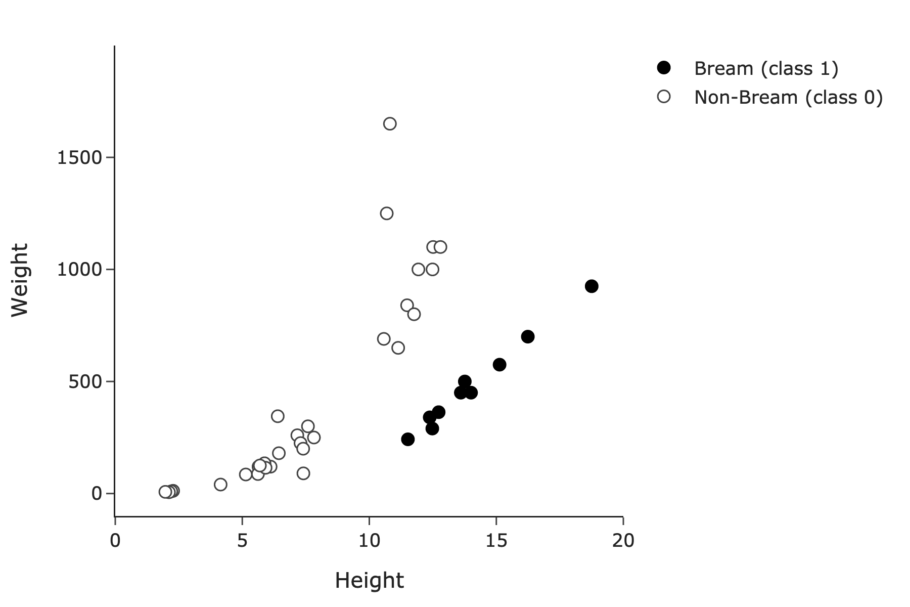
Suppose we use height only to predict species. In the 1-dimensional feature space, is the training set linearly separable?
Yes
No
Answer: No.
There is no vertical line of the form x = c that separates the black points from the outlined points.
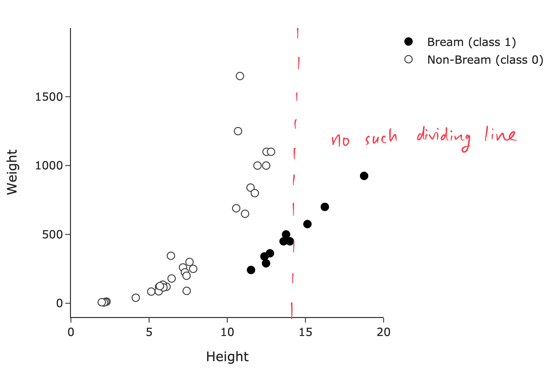
We’re searching for a vertical line, because we’re using height only to predict species, and with just one feature, we must consider if the data is separable using a line in a d = 1 dimensional plot, i.e. on a number line.
The average score on this problem was 90%.
Suppose we use both height and weight to predict species. In the 2-dimensional feature space, is the training set linearly separable?
Yes
No
Answer: Yes.
Here, we’re using d = 2 features, so we’re searching for a line in the 2-dimensional feature space that separates the two classes perfectly.
And indeed, you can draw a sloped line of the form y = mx + b – or more precisely, \text{weight} = m \cdot \text{height} + b – that separates the black points from the outlined points. One such line is shown below:
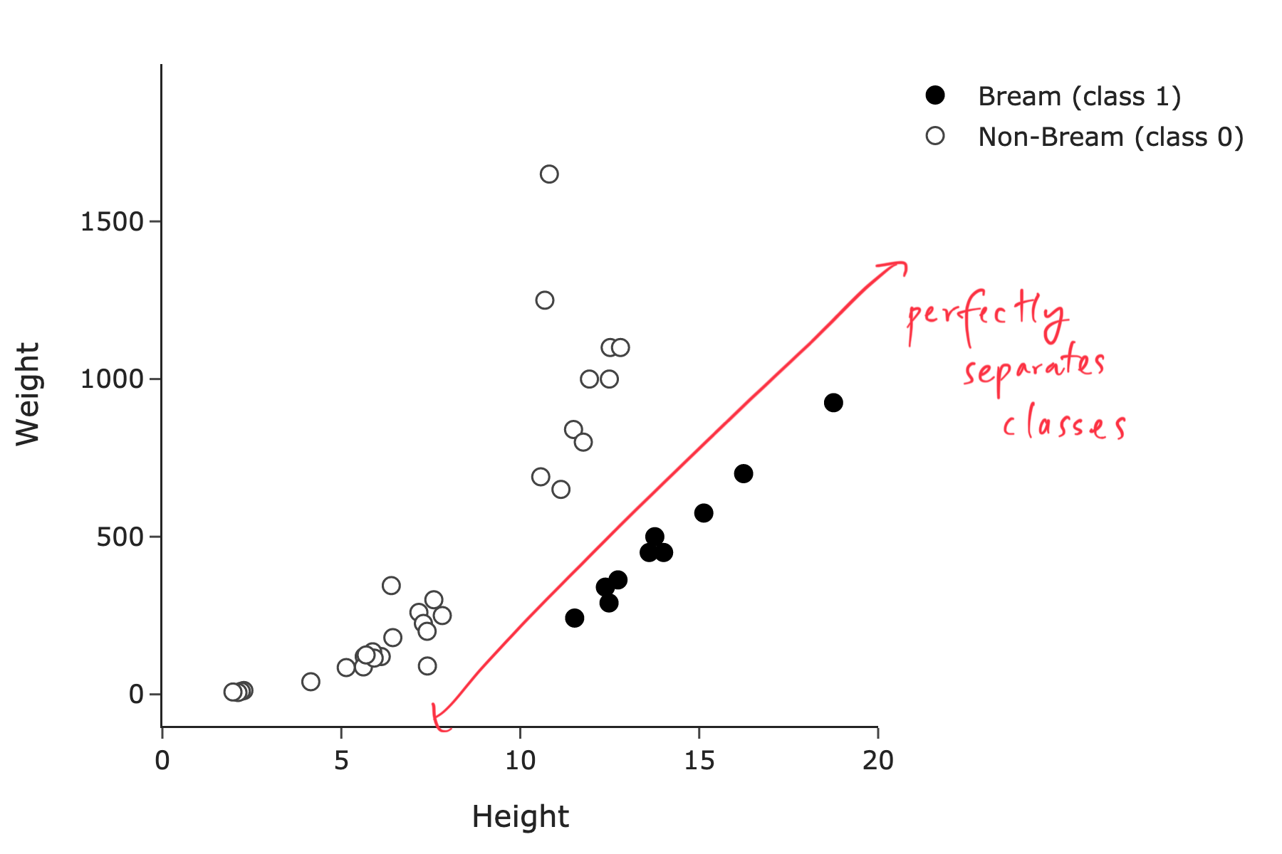
The average score on this problem was 92%.
Suppose we use both height and weight to predict species. What is minimum depth d required for a decision tree classifier to achieve a training accuracy of 100%?
1
2
3
4
5
10
40
Answer: 2.
See the decision boundary below:
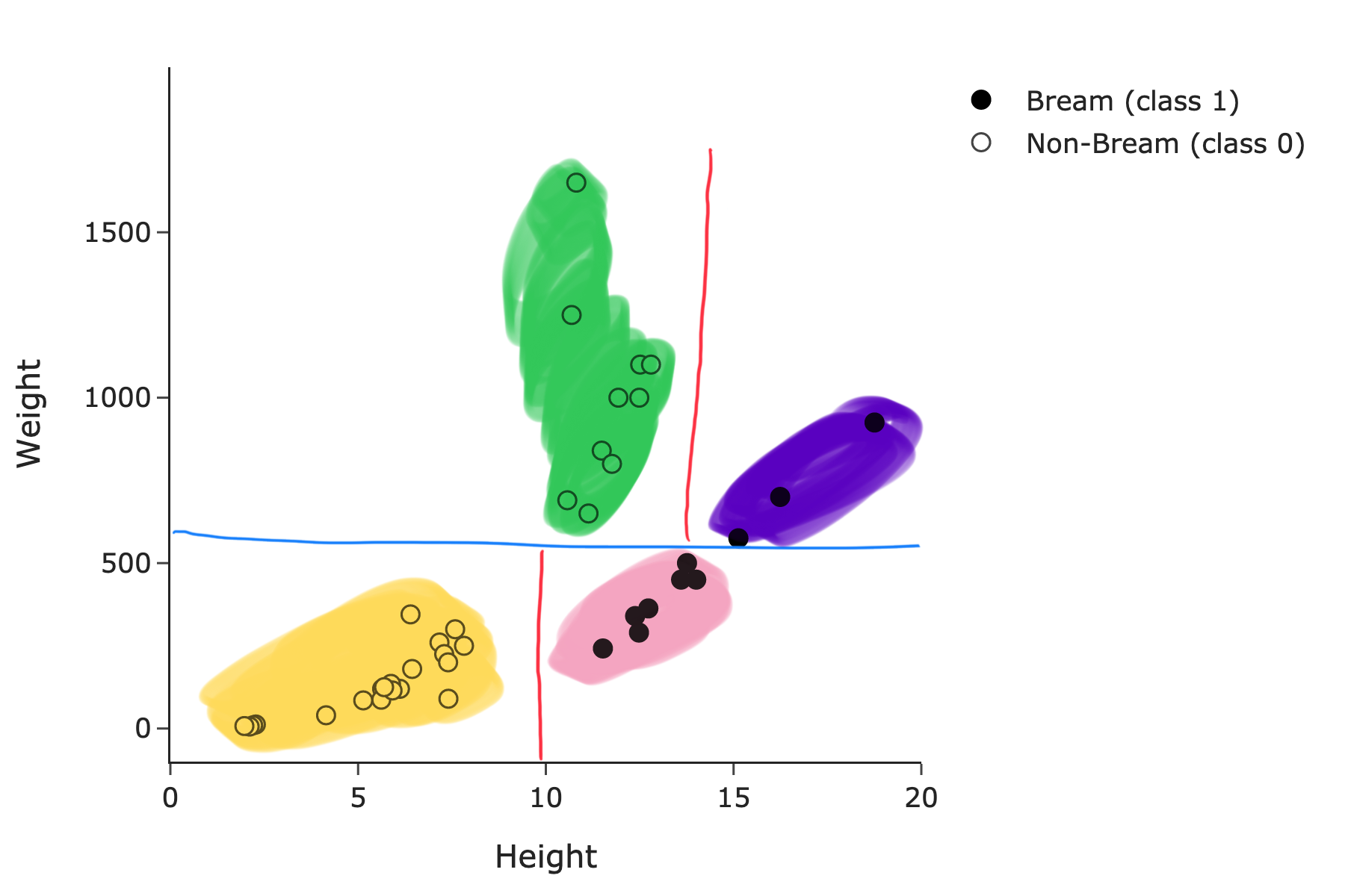
The resulting fit decision tree would be:
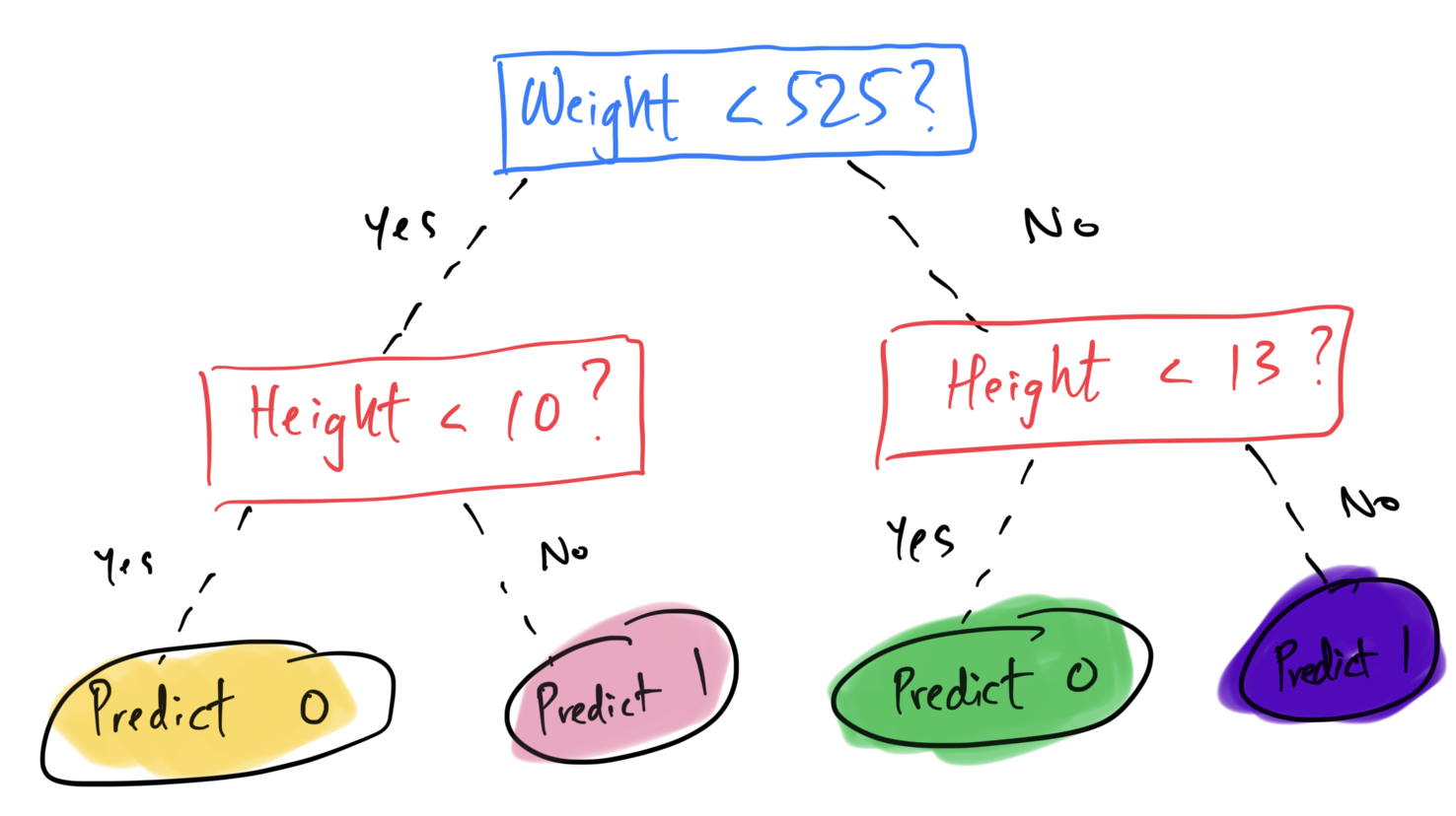
This tree only needs to ask a maximum of 2 questions to classify any point in the training set correctly.
The average score on this problem was 64%.
Suppose we use both height and weight to predict species. If we use a k-nearest neighbors classifier with k=1, which class would be predicted for a fish with height 20 and weight 1250?
Class 1 (Bream)
Class 0 (non-Bream)
Answer: Class 0 (non-Bream).
Given that k = 1, we classify this new fish as having the same class as one nearest neighbor to it in the training set. The nearest neighbor to this new fish is the fish with height 10 and weight 1250, which is a non-Bream fish. This result is a little counterintuitive at first glance – it looks like the closest neighbor is a black point (Bream) – but pay attention to the scale of the axes!
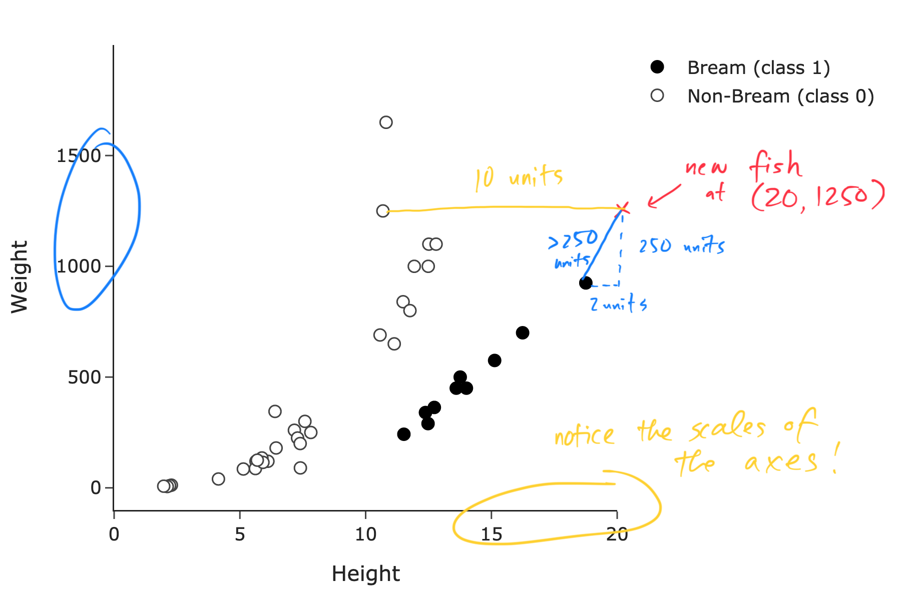
The average score on this problem was 14%.
For your convenience, we show the training set of n=40 points again below, in which 10 points belong to class 1.
Suppose we use height (x_i) only to predict species. If we use logistic regression without regularization, which option best describes the fit model, P(y_i = 1 | x_i)?
P(y_i = 1 | x_i) = \sigma \left(-15 - \frac{2}{3}x_i \right)
P(y_i = 1 | x_i) = \sigma \left(-15 + \frac{2}{3}x_i \right)
P(y_i = 1 | x_i) = \sigma \left(-20 + \frac{2}{3}x_i \right)
P(y_i = 1 | x_i) = \sigma \left(-15 - \frac{5}{4}x_i \right)
P(y_i = 1 | x_i) = \sigma \left(-15 + \frac{5}{4}x_i \right)
P(y_i = 1 | x_i) = \sigma \left(-20 + \frac{5}{4}x_i \right)
Answer: P(y_i = 1 | x_i) = \sigma \left(-15 + \frac{5}{4}x_i \right)
Firstly, we can rule out any option with a negative coefficient on x_i. This is because the frequency of Bream fish increases as height increases, so the probability of a Bream fish should increase as height increases. (Remember that \sigma(t) is an increasing function of t.)
When deciding between the remaining options, we can use the fact that \sigma(0) = \frac{1}{2}. Intuitively, the predicted probability that a fish is a Bream fish should be \frac{1}{2} in the “middle” of the data, when we are seeing equally many Bream and non-Bream fish. This roughly occurs around a height of 12.
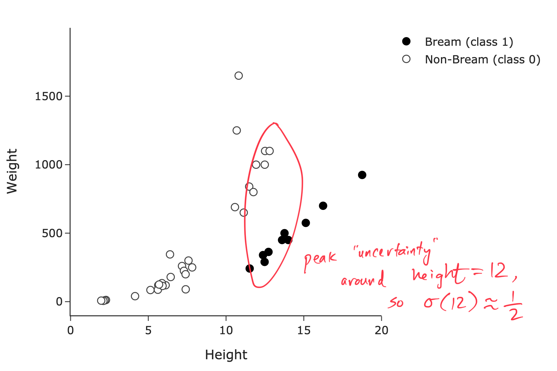
If we consider the four options that have positive coefficients on x_i and solve for x_i when P(y_i = 1 | x_i) = \frac{1}{2}, we get the following:
So, we choose P(y_i = 1 | x_i) = \sigma \left(-15 + \frac{5}{4}x_i \right).
The average score on this problem was 64%.
Suppose we use height (x_i) only to predict species. If we use L_2-regularized logistic regression with a regularization hyperparameter of \lambda = 10^{10}, what is the value of w_0^* in the fit model P(y_i = 1 | x_i) = \sigma(w_0^* + w_1^*x_i)?
3
1 / 3
4
1 / 4
\log \left( 3 \right)
\log \left( 1 / 3 \right)
\log \left( 4 \right)
\log \left( 1 / 4 \right)
Answer: \log \left( 1 / 3 \right).
If we let \lambda \rightarrow \infty in the regularized objective function, the value of w_1^* is forced to 0. However, the value of w_0^* is not constrained, since we don’t regularize the intercept term. Instead, our model will be of the form:
P(y_i = 1 | x_i) = \sigma(w_0^*)
Independent of the value of x_i, the probability that a fish is of species Bream is \frac{1}{4}, since 10 of the 40 points in the training set correspond to Bream fish. So, we have:
\frac{1}{4} = \sigma(w_0^*)
Now, we must solve for w_0^* in the equation above. To do so, we use the fact that if y = \sigma(x), then x = \log \left( \frac{y}{1 - y} \right). So, we have:
w_0^* = \log \left( \frac{\frac{1}{4}}{1 - \frac{1}{4}} \right) = \log \left( 1 / 3 \right)
So, the value of w_0^* is \boxed{\log \left( 1 / 3 \right)}.
The average score on this problem was 34%.
For the rest of this question, suppose we use both height and weight to predict species. Suppose we use logistic regression — possibly with regularization — and choose a classification threshold of T, where 0 \leq T \leq 1. The resulting decision boundary is shown below, along with the same training set as before (which has n=40 points, 10 of which belong to class 1).
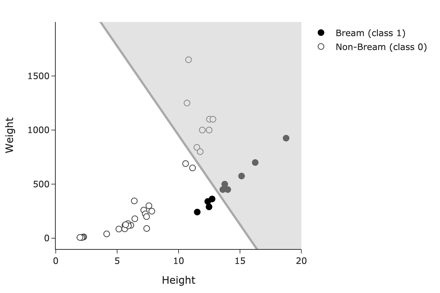
In the region above the line, shaded gray, our classifier predicts class 1 (Bream); in the region below the line, our classifier predicts class 0 (non-Bream).
Was regularization used when fitting the logistic regression model whose decision boundary is shown above?
Yes, regularization was used
No, regularization was not used
Answer: Yes, regularization was used.
If regularization wasn’t used, the decision boundary would look much closer to the line shown in Problem 8.2’s solution, which has very high training accuracy. This line is much worse than that one, and so it must have been regularized. (Some regularization is necessary since the dataset is linearly separable, but in practice to fit this data, we’d have used a much smaller regularization hyperparameter than the one that was used here.)
The average score on this problem was 47%.
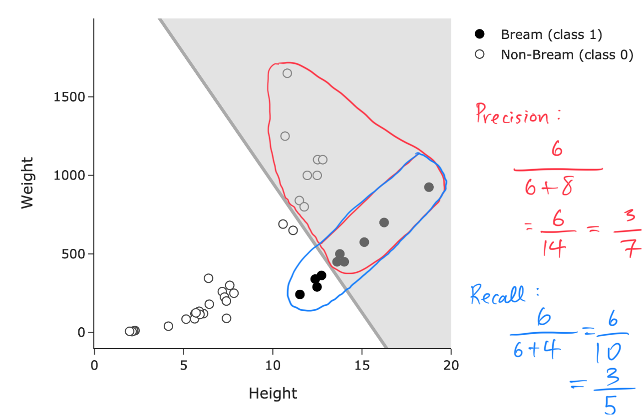
What are the precision and recall of the classifier above? Give your answers as simplified fractions. Answers that “swap" precision and recall will not be given any credit.
Answer: Precision = \frac{3}{7}, Recall = \frac{3}{5}.
Recall (no pun intended), we have that:
\text{Precision} = \frac{\text{True Positives}}{\text{True Positives} + \text{False Positives}}
\text{Recall} = \frac{\text{True Positives}}{\text{True Positives} + \text{False Negatives}}
Here: - A true positive is a Bream fish that was correctly classified as a Bream fish (a black point in the shaded area), of which there are 6. - A false positive is a non-Bream fish that was incorrectly classified as a Bream fish (an outlined point in the shaded area), of which there are 8. - A false negative is a Bream fish that was incorrectly classified as a non-Bream fish (a black point in the non-shaded area), of which there are 4.
So, we have:
\text{Precision} = \frac{6}{6 + 8} = \frac{6}{14} = \frac{3}{7}
\text{Recall} = \frac{6}{6 + 4} = \frac{6}{10} = \frac{3}{5}
The average score on this problem was 75%.
Suppose that each time we accidentally misclassify a fish’s species as Bream, we must pay a fine to the local aquarium. Given this fact alone, is it more important for our classifier to have high precision or high recall?
High precision
High recall
Answer: High precision.
Here, we’re being penalized for misclassifying a Bream fish as a non-Bream fish. So, we want to minimize the number of false positives. Since precision decreases as the number of false positives increases, we want to maximize precision.
The average score on this problem was 88%.
Consider a dataset of n non-negative numbers, x_1 < x_2 < \ldots < x_n, that are evenly spaced. In other words, x_{i+1} - x_i is some fixed positive constant, for all i = 1, 2, ..., n-1. Furthermore, assume that n is an even integer that is not a multiple of 4.
We’d like to use k-means clustering to cluster this dataset into k = 2 clusters, Cluster 1 and Cluster 2, defined by two centroids, \mu_1 and \mu_2, respectively.
Suppose we initialize the two centroids at \mu_1 = x_1 and \mu_2 = x_2.
In iteration 1, before updating the locations of the centroids, how many points belong to each cluster? Give your answers in the form of expressions involving n and/or constants.
Answer:
The average score on this problem was 77%.
In iteration 1, after updating the locations of the centroids, both centroids are located exactly at values in the dataset. Which data point is each centroid now located at? Give your answers in the form of expressions involving n and/or constants, but not x. (For example, if you believe \mu_2 is now located at x_{n-1}, put n-1 in the second box.)
\mu_1 is now located at x_p, where p = \hspace{0.05in}
\mu_2 is now located at x_q, where q =
Answer:
The average score on this problem was 75%.
In iteration 2, before updating the locations of the centroids, how many points belong to each cluster? Give your answers in the form of expressions involving n and/or constants.
Answer:
The average score on this problem was 43%.
In one English sentence, name and describe the objective function that k-means clustering minimizes.
Answer: The objective function that k-means clustering minimizes is called inertia, which is the sum of the squared distances between each point and the centroid closest to it.
The average score on this problem was 72%.