Final Review, Day 1 (Wednesday)

The problems in this worksheet are taken from past exams in similar classes. Work on them on paper, since the exams you take in this course will also be on paper.

We encourage you to attempt these problems before Wednesday’s exam review session, so that we have enough time to walk through the solutions to all of the problems.

We will enable the solutions here after the review session, though you can find the written solutions to these problems in other discussion worksheets.

While you can treat this as a mock exam of sorts, there are many topics that are in scope for the final exam that do not appear here, and this may not be representative of the length of the real Final Exam.

Problem 1

\vec{u} = \begin{bmatrix} 1 \\ 0 \\ 0 \end{bmatrix} \qquad \vec{v} = \begin{bmatrix} 0 \\ 1 \\ 1 \end{bmatrix}

We define X \in \mathbb{R}^{3 \times 2} to be the matrix whose first column is \vec u and whose second column is \vec v.

Problem 1.1

Find a scalar k such that \vec{y} is in \text{span}(\vec u, \vec v). Give your answer as a constant with no variables.

Answer: 252.

Vectors in \text{span}(\vec u, \vec v) are all linear combinations of \vec{u} and \vec{v}, meaning they have the form:

a \begin{bmatrix} 1 \\ 0 \\ 0 \end{bmatrix} + b \begin{bmatrix} 0 \\ 1 \\ 1 \end{bmatrix} = \begin{bmatrix} a \\ b \\ b \end{bmatrix}

From this, any vector in the span must have its second and third components equal. Since \vec{y} has its third component as 252, so k must equal to 252.

Problem 1.2

Show that: (X^TX)^{-1}X^T = \begin{bmatrix} 1 & 0 & 0 \\ 0 & \frac{1}{2} & \frac{1}{2} \end{bmatrix}

Hint: If A = \begin{bmatrix} a_1 & 0 \\ 0 & a_2 \end{bmatrix}, then A^{-1} = \begin{bmatrix} \frac{1}{a_1} & 0 \\ 0 & \frac{1}{a_2} \end{bmatrix}.

Answer: We can construct the following series of matrices to get (X^TX)^{-1}X^T.

X = \begin{bmatrix} 1 & 0 \\ 0 & 1 \\ 0 & 1 \end{bmatrix}
X^T = \begin{bmatrix} 1 & 0 & 0 \\ 0 & 1 & 1 \end{bmatrix}
X^TX = \begin{bmatrix} 1 & 0 \\ 0 & 2 \end{bmatrix}
(X^TX)^{-1} = \begin{bmatrix} 1 & 0 \\ 0 & \frac{1}{2} \end{bmatrix}
(X^TX)^{-1}X^T = \begin{bmatrix} 1 & 0 & 0 \\ 0 & \frac{1}{2} & \frac{1}{2} \end{bmatrix}

Problem 1.3

Find scalars a and b such that a \vec u + b \vec v is the vector in \text{span}(\vec u, \vec v) that is as close to \vec{y} as possible. Give your answers as constants with no variables.

Answer: a = 4, b = 5.

The result from the part (b) implies that when using the normal equations to find coefficients for \vec u and \vec v – which we know from lecture produce an error vector whose length is minimized – the coefficient on \vec u must be y_1 and the coefficient on \vec v must be \frac{y_2 + y_3}{2}. This can be shown by taking the result from part (b), \begin{bmatrix} 1 & 0 & 0 \\ 0 & \frac{1}{2} & \frac{1}{2} \end{bmatrix}, and multiplying it by the vector \vec y = \begin{bmatrix} y_1 \\ y_2 \\ y_3 \end{bmatrix}.

Here, y_1 = 4, so a = 4. We also know y_2 = 2 and y_3 = 8, so b = \frac{2+8}{2} = 5.

Problem 1.4

Let \vec{e} = \vec{y} - (a \vec u + b \vec v), where a and b are the values you found in part (c).

Answer: 3 \sqrt{2}.

The correct value of a \vec u + b \vec v = \begin{bmatrix} 4 \\ 5 \\ 5\end{bmatrix}. Then, \vec{e} = \begin{bmatrix} 4 \\ 2 \\ 8 \end{bmatrix} - \begin{bmatrix} 4 \\ 5 \\ 5 \end{bmatrix} = \begin{bmatrix} 0 \\ -3 \\ 3 \end{bmatrix}, which has a length of \sqrt{0^2 + (-3)^2 + 3^2} = 3\sqrt{2}.

Problem 1.5

Is it true that, for any vector \vec{y} \in \mathbb{R}^3, we can find scalars c and d such that the sum of the entries in the vector \vec{y} - (c \vec u + d \vec v) is 0?

Answer: Yes, but for a reason that isn’t listed here.

Here’s the full reason:

We can use the normal equations to find c and d, no matter what \vec{y} is.
The error vector \vec e that results from using the normal equations is such that \vec e is orthogonal to the span of the columns of X.
The columns of X are just \vec u and \vec v. So, \vec e is orthogonal to any linear combination of \vec u and \vec v.
One of the many linear combinations of \vec u and \vec v is \begin{bmatrix} 1 \\ 0 \\ 0 \end{bmatrix} + \begin{bmatrix} 0 \\ 1 \\ 1 \end{bmatrix} = \begin{bmatrix} 1 \\ 1 \\ 1 \end{bmatrix}.
This means that the vector \vec e is orthogonal to \begin{bmatrix} 1 \\ 1 \\ 1 \end{bmatrix}, which means that \vec{1}^T \vec{e} = 0 \implies \sum_{i = 1}^3 e_i = 0.

Problem 1.6

Suppose that Q \in \mathbb{R}^{100 \times 12}, \vec{s} \in \mathbb{R}^{100}, and \vec{f} \in \mathbb{R}^{12}. What are the dimensions of the following product?

Answer: Scalar.

\vec{s}^T: 1 x 100
Q: 100 x 12.
\vec{f}: 12 x 1.

The inner dimensions of 100 and 12 cancel, and so \vec{s}^T Q \vec{f} is of shape 1 x 1.

Problem 2

One piece of information that may be useful as a feature is the proportion of SAT test takers in a state in a given year that qualify for free lunches in school. The Series lunch_props contains 8 values, each of which are either "low", "medium", or "high". Since we can’t use strings as features in a model, we decide to encode these strings using the following Pipeline:

After calling pl.fit(lunch_props), pl.transform(lunch_props) evaluates to the following array:

and pl.named_steps["ohe"].get_feature_names() evaluates to the following array:

Given the above information, we can conclude that lunch_props has (a) value(s) equal to "low", (b) value(s) equal to "medium", and (c) value(s) equal to "high". (Note: Each of (a), (b), and (c) should be positive numbers, such that together, they add to 8.)

Answer: 3, 1, 4

The first column of the transformed array corresponds to the standardized one-hot-encoded low column. There are 3 values that are positive, which means there are 3 values that were originally 1 in that column pre-standardization. This means that 3 of the values in lunch_props were originally "low".

The second column of the transformed array corresponds to the standardized one-hot-encoded med column. There is only 1 value in the transformed column that is positive, which means only 1 of the values in lunch_props was originally "medium".

The Series lunch_props has 8 values, 3 of which were identified as "low" in subpart 1, and 1 of which was identified as "medium" in subpart 2. The number of values being "high" must therefore be 8 - 3 - 1 = 4.

Problem 3

Suppose we have one qualitative variable that that we convert to numerical values using one- hot encoding. We’ve shown the first four rows of the resulting design matrix below:

Problem 3.1

Say we train a linear model m_1 on these data. Then, we replace all of the 1 values in column a with 3’s and all of the 1 values in column b with 2’s and train a new linear model m_2. Neither m_1 nor m_2 have an intercept term. On the training data, the average squared loss for m_1 will be ________ that of m_2.

Answers:

The answer is equal to.

Because we can simply adjust the weights in the opposite way that we rescale the one-hot columns, any model obtainable with the original encoding can also be obtained with the rescaled encoding. This guarantees that the training loss remains unchanged.

When one-hot encoding is used, each category is represented by a column that typically contains only 0s and 1s. Rescaling these columns means multiplying the 1s by a constant (for example, turning 1 into 2 or 3). However, if we also adjust the corresponding weights in the model by dividing by that same constant, the product of the rescaled column value and its weight remains the same. Since the model’s predictions are based on these products, the predictions will not change, and as a result, the average squared loss on the training data will also remain unchanged.

For example, let us say we have categorical variable “Color” with three levels: Red, Green, and Blue. We one-hot encode this variable into three columns. For an observation: - If the color is Red, the encoded values might be: Red = 1, Green = 0, Blue = 0.

Now, suppose we decide to multiply the column for Red by 2. The new value for a Red observation becomes 2 instead of 1. To keep the prediction the same, we can simply use half the weight for this column in the model. This inverse adjustment ensures that the final product (column value multiplied by weight) remains unchanged. Thus, the model’s prediction and the average squared loss on the training data stay the same.

Problem 3.2

To account for the intercept term, we add a column of all ones to our design matrix from part a. That is, the resulting design matrix has four columns: a with 3’s instead of 1’s, b with 2’s instead of 1’s, c, and a column of all ones. What is the rank of the new design matrix with these four columns?

Answers:

The answer is 3.

Note that the column c = intercept column −\frac{1}{3}a + \frac{1}{2}b. Hence, there is a linear dependence relationship, meaning that one of the columns is redundant and that the rank of the new design matrix is 3.

Problem 4

Suppose we build a binary classifier that uses a song’s "track_name" and "artist_names" to predict whether its genre is "Hip-Hop/Rap" (1) or not (0).

For our classifier, we decide to use a brand-new model built into sklearn called the
BillyClassifier. A BillyClassifier instance has three hyperparameters that we’d like to tune. Below, we show a dictionary containing the values for each hyperparameter that we’d like to try:

To find the best combination of hyperparameters for our BillyClassifier, we first conduct a train-test split, which we use to create a training set with 800 rows. We then use GridSearchCV to conduct k-fold cross-validation for each combination of hyperparameters in hyp_grid, with k=4.

Problem 4.1

When we call GridSearchCV, how many times is a BillyClassifier instance trained in total? Give your answer as an integer.

Answer: 2400

There are 12 \cdot 10 \cdot 5 = 600 combinations of hyperparameters. For each combination of hyperparameters, we will train a BillyClassifier with that combination of hyperparameters k = 4 times. So, the total number of BillyClassifier instances that will be trained is 600 \cdot 4 = 2400.

Problem 4.2

In each of the 4 folds of the data, how large is the training set, and how large is the validation set? Give your answers as integers.

Answer: 600, 200

Since we performed k=4 cross-validation, we must divide the training set into four disjoint groups each of the same size. \frac{800}{4} = 200, so each group is of size 200. Each time we perform cross validation, one group is used for validation, and the other three are used for training, so the validation set size is 200 and the training set size is 200 \cdot 3 = 600.

Problem 4.3

Suppose that after fitting a GridSearchCV instance, its best_params_ attribute is

Answer: Option B

When performing cross validation, we select the combination of hyperparameters that had the highest average validation accuracy across all four folds of the data. That is, by definition, how best_params_ came to be. None of the other options are guaranteed to be true.

Problem 5

Suppose we want to use LASSO (i.e. minimize mean squared error with L_1 regularization) to fit a linear model that predicts the number of ingredients in a product given its price and rating.

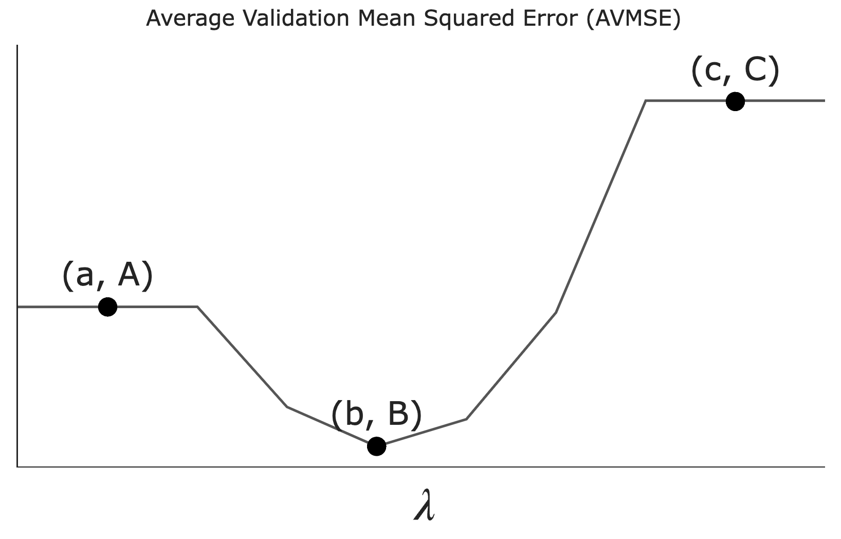
Let \lambda be a non-negative regularization hyperparameter. Using cross-validation, we determine the average validation mean squared error — which we’ll refer to as AVMSE in this question — for several different choices of \lambda. The results are given below.

Problem 5.1

Answer: Model complexity and model variance both decrease.

As \lambda increases, the L_1 regularization penalizes larger coefficient values more heavily, forcing the model to forget the details in the training data and focus on the bigger picture. This effectively reduces the number of non-zero coefficients, decreasing model complexity. Since model complexity and model variance are the same thing, variance also decreases.

Problem 5.2

Answer: The AVMSE of an unregularized multiple linear regression model.

Point A represents the case where \lambda = 0, meaning no regularization is applied. This corresponds to an unregularized multiple linear regression model.

Problem 5.3

Answer: The AVMSE of the \lambda we’d choose to use to train a model.

Point B is the minimum point on the graph, indicating the optimal \lambda value that minimizes the AVMSE. This is because we don’t typically regularize the intercept term’s coefficient, w_0^*.

Problem 5.4

Answer: The AVMSE of the constant model.

Point C represents the AVMSE when \lambda is very large, effectively forcing all coefficients to zero. This corresponds to the constant model.

Problem 6

Problem 6.1

Without using gradient descent or calculus, what is the value h^* that minimizes R(h)?

h^* = -1

The minimum possible value of the exponent is 0, since anything squared is non-negative. The exponent is 0 when (x+1)^2 = 0, i.e. when x = -1. Since e^{(x+1)^2} gets larger as (x+1)^2 gets larger, the minimizing input h^* is -1.

Problem 6.2

Now, suppose we want to use gradient descent to minimize R(h). Assume we use an initial guess of h^{(0)} = 0. What is h^{(1)}? Give your answer in terms of a generic step size, \alpha, and other constants. (e is a constant.)

h^{(1)} = -\alpha \cdot 2e

First, we find \frac{dR}{dh}(h):

\frac{dR}{dh}(h) = 2(h+1) e^{(h+1)^2}

Then, we know that

h^{(1)} = h^{(0)} - \alpha \frac{dR}{dh}(h^{(0)}) = 0 - \alpha \frac{dR}{dh}(0)

In our case, \frac{dR}{dh}(0) = 2(0 + 1) e^{(0+1)^2} = 2e, so

h^{(1)} = -\alpha \cdot 2e

Problem 6.3

Using your answers from the previous two parts, what should we set the value of \alpha to be if we want to ensure that gradient descent finds h^* after just one iteration?

\alpha = \frac{1}{2e}

We know from the part 2 that h^{(1)} = -\alpha \cdot 2e, and we know from part 1 that h^* = -1. If gradient descent converges in one iteration, that means that h^{(1)} = h^*; solving this yields

-\alpha \cdot 2e = -1 \implies \alpha = \frac{1}{2e}

Problem 6.4

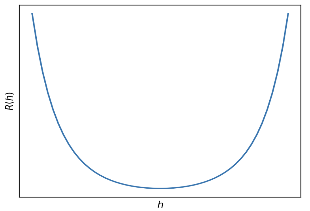
True or False: Given an appropriate choice of step size, \alpha, gradient descent is guaranteed to find the minimizer of R(h).

True.

R(h) is convex, since the graph is bowl shaped. (It can also be proved that R(h) is convex using the second derivative test.) It is also differentiable, as we saw in part 2. As a result, since it’s both convex and differentiable, gradient descent is guaranteed to be able to minimize it given an appropriate choice of step size.

Problem 7

We decide to build a classifier that takes in a state’s demographic information and predicts whether, in a given year:

Problem 7.1

The simplest possible classifier we could build is one that predicts the same label (1 or 0) every time, independent of all other features.

If a > b, then the constant classifier that maximizes training accuracy predicts 1 every time; otherwise, it predicts 0 every time.

For which combination of a and b is the above statement not guaranteed to be true?

Answer: Option 2

Conceptually, we’re looking for a combination of a and b such that when a > b, it’s true that in more than 50% of states, the "Math" value is larger than the "Verbal" value. Let’s look at all four options through this lens:

Option 1: sat['Math'] > sat['Verbal'] is a Series of Boolean values, containing True for all states where the "Math" value is larger than the "Verbal" value and False for all other states. The mean of this series, then, is the proportion of states satisfying this criteria, and since b is 0.5, a > b is True only when the bolded condition above is True.
Option 3 is the same as Option 1 – note that x > y is equivalent to x - y > 0.
Option 4: sat['Math'] / sat['Verbal'] is a Series that contains values greater than 1 whenever a state’s "Math" value is larger than its "Verbal" value and less than or equal to 1 in all other cases. As in the other options that work, (sat['Math'] / sat['Verbal']) > 1 is a Boolean Series with True for all states with a larger "Math" value than "Verbal" values; a > b compares the proportion of True values in this Series to 0.5. (Here, p - 0.5 > 0 is the same as p > 0.5.)

Then, by process of elimination, Option 2 must be the correct option – that is, it must be the only option that doesn’t work. But why? sat['Math'] - sat['Verbal'] is a Series containing the difference between each state’s "Math" and "Verbal" values, and .mean() computes the mean of these differences. The issue is that here, we don’t care about how different each state’s "Math" and "Verbal" values are; rather, we just care about the proportion of states with a bigger "Math" value than "Verbal" value. It could be the case that 90% of states have a larger "Math" value than "Verbal" value, but one state has such a big "Verbal" value that it makes the mean difference between "Math" and "Verbal" scores negative. (A property you’ll learn about in future probability courses is that this is equal to the difference in the mean "Math" value for all states and the mean "Verbal" value for all states – this is called the “linearity of expectation” – but you don’t need to know that to answer this question.)

Problem 7.2

Suppose we train a classifier, named Classifier 1, and it achieves an accuracy of \frac{5}{9} on our training set.

Typically, root mean squared error (RMSE) is used as a performance metric for regression models, but mathematically, nothing is stopping us from using it as a performance metric for classification models as well.

What is the RMSE of Classifier 1 on our training set? Give your answer as a simplified fraction.

Answer: \frac{2}{3}

An accuracy of \frac{5}{9} means that the model is such that out of 9 values, 5 are labeled correctly. By extension, this means that 4 out of 9 are not labeled correctly as 0 or 1.

Remember, RMSE is defined as

\text{RMSE} = \sqrt{\frac{1}{n} \sum_{i = 1}^n (y_i - H(x_i))^2}

where y_i represents the ith actual value and H(x_i) represents the ith prediction. Here, y_i is either 0 or 1 and $H(x_i) is also either 0 or 1. We’re told that \frac{5}{9} of the time, y_i and H(x_i) are the same; in those cases, (y_i - H(x_i))^2 = 0^2 = 0. We’re also told that \frac{4}{9} of the time, y_i and H(x_i) are different; in those cases, (y_i - H(x_i))^2 = 1. So,

\text{RMSE} = \sqrt{\frac{5}{9} \cdot 0 + \frac{4}{9} \cdot 1} = \sqrt{\frac{4}{9}} = \frac{2}{3}

Problem 7.3

While Classifier 1’s accuracy on our training set is \frac{5}{9}, its accuracy on our test set is \frac{1}{4}. Which of the following scenarios is most likely?

Answer: Option 2

Since the accuracy of Classifier 1 is much higher on the dataset used to train it than the dataset it was tested on, it’s likely Classifer 1 overfit to the training set because it was too complex. To fix the issue, we need to decrease its complexity, so that it focuses on learning the general structure of the data in the training set and not too much on the random noise in the training set.

For the remainder of this question, suppose we train another classifier, named Classifier 2, again on our training set. Its performance on the training set is described in the confusion matrix below. Note that the columns of the confusion matrix have been separately normalized so that each has a sum of 1.

Problem 7.4

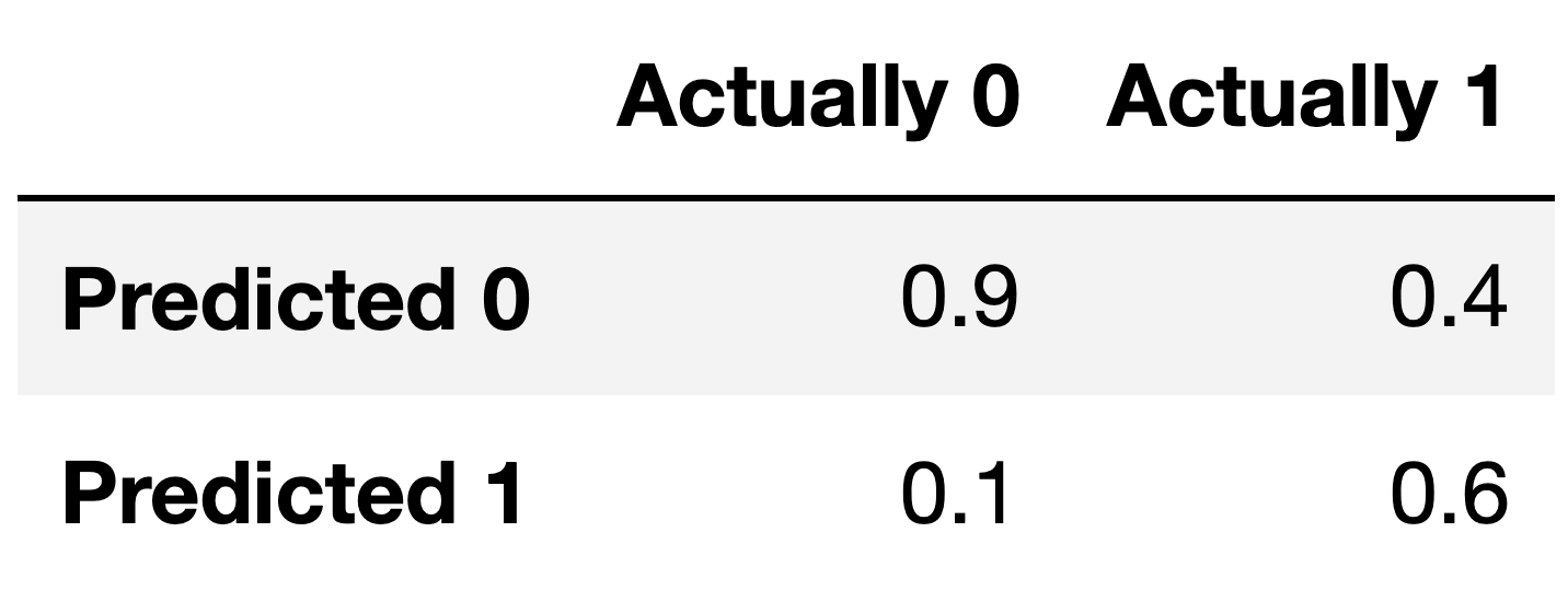
Suppose conf is the DataFrame above. Which of the following evaluates to a Series of length 2 whose only unique value is the number 1?

Answer: Option 1

Note that the columns of conf sum to 1 – 0.9 + 0.1 = 1, and 0.4 + 0.6 = 1. To create a Series with just the value 1, then, we need to sum the columns of conf, which we can do using conf.sum(axis=0). conf.sum(axis=1) would sum the rows of conf.

Problem 7.5

Answer: recall

The number 0.6 appears in the bottom-right corner of conf. Since conf is column-normalized, the value 0.6 represents the proportion of values in the second column that were predicted to be 1. The second column contains values that were actually 1, so 0.6 is really the proportion of values that were actually 1 that were predicted to be 1, that is, \frac{\text{actually 1 and predicted 1}}{\text{actually 1}}. This is the definition of recall!

If you’d like to think in terms of true positives, etc., then remember that: - True Positives (TP) are values that were actually 1 and were predicted to be 1. - True Negatives (TN) are values that were actually 0 and were predicted to be 0. - False Positives (FP) are values that were actually 0 and were predicted to be 1. - False Negatives (FN) are values that were actually 1 and were predicted to be 0.

Recall is \frac{\text{TP}}{\text{TP} + \text{FN}}.

For your convenience, we show the column-normalized confusion matrix from the previous page below. You will need to use the specific numbers in this matrix when answering the following subpart.

Problem 7.6

Suppose a fraction \alpha of the labels in the training set are actually 1 and the remaining 1 - \alpha are actually 0. The accuracy of Classifier 2 is 0.65. What is the value of \alpha?

Answer: \frac{5}{6}

Here is one way to solve this problem:

accuracy = \frac{TP + TN}{TP + TN + FP + FN}

Given the values from the confusion matrix:

accuracy = \frac{0.6 \cdot \alpha + 0.9 \cdot (1 - \alpha)}{\alpha + (1 - \alpha)}
accuracy = \frac{0.6 \cdot \alpha + 0.9 - 0.9 \cdot \alpha}{1}
accuracy = 0.9 - 0.3 \cdot \alpha

Therefore:

0.65 = 0.9 - 0.3 \cdot \alpha
0.3 \cdot \alpha = 0.9 - 0.65
0.3 \cdot \alpha = 0.25
\alpha = \frac{0.25}{0.3}
\alpha = \frac{5}{6}

Problem 8

Suppose we fit a logistic regression model that predicts whether a product is designed for sensitive skin, given its price, x^{(1)}, number of ingredients, x^{(2)}, and rating, x^{(3)}. After minimizing average cross-entropy loss, the optimal parameter vector is as follows:

In other words, the intercept term is -1, the coefficient on price is \frac{1}{5}, the coefficient on the number of ingredients is -\frac{3}{5}, and the coefficient on rating is 0.

Which of the following products have a predicted probability of being designed for sensitive skin of at least 0.5 (50%)? For each product, select Yes or No.

Using the logistic function, we can predict the probability that a product is designed for sensitive skin using:

P(y_i = 1 | \vec{x}_i) = \sigma(\vec w^* \cdot \text{Aug} (\vec x_i) )

where \sigma(t) = \frac{1}{1 + e^{-t}} is the sigmoid function.

One of the properties we discussed in Lecture 22 was that \sigma(0) = \frac{1}{2}, meaning that if the input to \sigma(\cdot) is greater than or equal to 0, the predicted probability is greater than or equal to \frac{1}{2}. So, the problem here reduces to computing \vec w^* \cdot \text{Aug} (\vec x_i) for all four products, and checking whether this dot product is \geq 0.

Wolfcare:

\vec w^* \cdot \text{Aug} (\vec x_\text{Wolfcare}) = \begin{bmatrix} -1 \\ \frac{1}{5} \\ -\frac{3}{5} \\ 0 \end{bmatrix} \cdot \begin{bmatrix} 1 \\ 15 \\ 20 \\ 4.5 \end{bmatrix} = -1 + \frac{1}{5}(15) - \frac{3}{5}(20) + 0 = -1 + 3 - 12 = -10

Since -10 < 0, P(y_\text{Wolfcare} = 1 | \vec{x}_\text{Wolfcare}) < \frac{1}{2}, so the answer is \boxed{\text{No}}.

Go Blue Glow:

\begin{align*} \vec w^* \cdot \text{Aug} (\vec x_\text{Go Blue Glow}) &= \begin{bmatrix} -1 \\ \frac{1}{5} \\ -\frac{3}{5} \\ 0 \end{bmatrix} \cdot \begin{bmatrix} 1 \\ 25 \\ 5 \\ 4.9 \end{bmatrix} \\ &= -1 + \frac{1}{5}(25) - \frac{3}{5}(5) + 0 = -1 + 5 - 3 = 1 \end{align*}

Since 1 > 0, P(y_\text{Go Blue Glow} = 1 | \vec{x}_\text{Go Blue Glow}) > \frac{1}{2}, so the answer is \boxed{\text{Yes}}.

DataSPF:

\begin{align*} \vec w^* \cdot \text{Aug} (\vec x_\text{DataSPF}) &= \begin{bmatrix} -1 \\ \frac{1}{5} \\ -\frac{3}{5} \\ 0 \end{bmatrix} \cdot \begin{bmatrix} 1 \\ 50 \\ 15 \\ 3.6 \end{bmatrix} \\ &= -1 + \frac{1}{5}(50) - \frac{3}{5}(15) + 0 = -1 + 10 - 9 = 0 \end{align*}

Since \vec w^* \cdot \text{Aug} (\vec x_\text{DataSPF})= 0, P(y_\text{DataSPF} = 1 | \vec{x}_\text{DataSPF}) = \frac{1}{2}, so the answer is \boxed{\text{Yes}}.

Maize Mist: \begin{align*} \vec w^* \cdot \text{Aug} (\vec x_\text{Maize Mist}) &= \begin{bmatrix} -1 \\ \frac{1}{5} \\ -\frac{3}{5} \\ 0 \end{bmatrix} \cdot \begin{bmatrix} 1 \\ 0 \\ 1 \\ 5.0 \end{bmatrix} \\ &= -1 + \frac{1}{5}(0) - \frac{3}{5}(1) + 0 = -1 - 0.6 = -1.6 \end{align*}

Since -1.6 < 0, P(y_\text{Maize Mist} = 1 | \vec{x}_\text{Maize Mist}) < \frac{1}{2}, so the answer is \boxed{\text{No}}.

Problem 9

Consider the following plot of data in d=2 dimensions. We’d like to use k-means clustering to cluster the data into k=3 clusters.

Suppose the crosses represent initial centroids, which are not themselves data points.

Problem 9.1

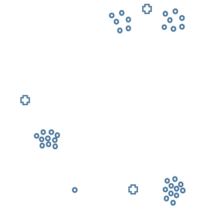
Which of the following facts are true about the cluster assignment during the first iteration, as determined by these initial centroids? Select all that apply.

Answer: Exactly two clusters contain at least 12 data points.

The top cluster will contain 13 data points.
The left cluster will contain 10 data points.
The bottom right cluster will contain 12 data points, including the outlier since it is closer to the bottom cross than to the left one.

Thus, the top cluster and bottom right clusters will contain at least 12 data points in Step 1 of the first iteration.

Problem 9.2

The cross shapes in the plot above represent positions of the initial centroids before the first iteration. Now the algorithm is run for one iteration, after which the centroids have been adjusted.

We are now starting the second iteration. Which of the following facts are true about the cluster assignment during the second iteration? Select all that apply.

Answers: Both of:

Exactly two clusters contain 11 data points.
Exactly one cluster contains at least 12 data points.

Let’s look at each cluster once again.

The top cluster will contain the same 13 data points as it did before the centroids were ever adjusted. All that happened in Step 2 of the first iteration was that the top centroid was moved down slightly, to the average x^{(2)} position of the 13 points up top.
The left cluster will contain 11 data points, including the one outlier. This is because, in Step 2 of the first iteration, the bottom right centroid moved to the right since it was pulled closer by the 11 non-outliers in the bottom right that were assigned to it in Step 1 of the first iteration. At the same time, the left centroid moved to the center of the group of 10 points in the left, since remember, the outlier belonged to the bottom right cluster in Step 1 of the first iteration.
- As a result, the outlier is now closer to the left centroid than the bottom right centroid, so it will be assigned to the left cluster in Step 1 of the second iteration.
The right cluster no longer possesses the outlier for the reasons described above, so the right cluster now just contains the bottom-right group of 11 data points.

So, the cluster sizes are 13, 11, and 11, which means that two of the clusters contain 11 data points and one of the clusters contains at least 12 data points.

Problem 9.3

Compare the value of inertia after the end of the second iteration to the value of inertia at the end of the first iteration. Which of the following facts are true? Select all that apply.

Problem 1

Problem 1.1

Click to view the solution.

Problem 1.2

Click to view the solution.

Problem 1.3

Click to view the solution.

Problem 1.4

Click to view the solution.

Problem 1.5

Click to view the solution.

Problem 1.6

Click to view the solution.

Problem 2

Click to view the solution.

Problem 3

Problem 3.1

Click to view the solution.

Problem 3.2

Click to view the solution.

Problem 4

Problem 4.1

Click to view the solution.

Problem 4.2

Click to view the solution.

Problem 4.3

Click to view the solution.

Problem 5

Problem 5.1

Click to view the solution.

Problem 5.2

Click to view the solution.

Problem 5.3

Click to view the solution.

Problem 5.4

Click to view the solution.

Problem 6

Problem 6.1

Click to view the solution.

Problem 6.2

Click to view the solution.

Problem 6.3

Click to view the solution.

Problem 6.4

Click to view the solution.

Problem 7

Problem 7.1

Click to view the solution.

Problem 7.2

Click to view the solution.

Problem 7.3

Click to view the solution.

Problem 7.4

Click to view the solution.

Problem 7.5

Click to view the solution.

Problem 7.6

Click to view the solution.

Problem 8

Click to view the solution.

Problem 9

Problem 9.1

Click to view the solution.

Problem 9.2

Click to view the solution.

Problem 9.3

Click to view the solution.

👋 Feedback: Find an error? Still confused? Have a suggestion? Let us know here.