Final Review, Day 2 (Saturday)

← return to study.practicaldsc.org

The problems in this worksheet are taken from past exams in similar classes. Work on them on paper, since the exams you take in this course will also be on paper.

We encourage you to attempt these problems before Saturday’s exam review session, so that we have enough time to walk through the solutions to all of the problems.

We will enable the solutions here after the review session, though you can find the written solutions to these problems in other discussion worksheets.

While you can treat this as a mock exam of sorts, there are many topics that are in scope for the final exam that do not appear here, and this may not be representative of the length of the real Final Exam.

Problem 1

Consider the dataset shown below.

Problem 1.1

We want to use multiple regression to fit a prediction rule of the form H(x_i^{(1)}, x_i^{(2)}, x_i^{(3)}) = w_0 + w_1 x_i^{(1)} x_i^{(3)} + w_2 (x_i^{(2)} - x_i^{(3)})^2. Write down the design matrix X and observation vector \vec{y} for this scenario. No justification needed.

Problem 1.2

For the X and \vec{y} that you have written down, let \vec{w} be the optimal parameter vector, which comes from solving the normal equations X^TX\vec{w}=X^T\vec{y}. Let \vec{e} = \vec{y} - X \vec{w} be the error vector, and let e_i be the ith component of this error vector. Show that 4e_1+e_2+4e_3+e_4=0.

Problem 2

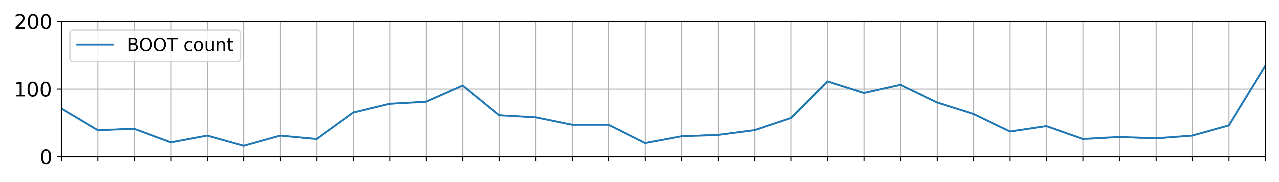
The two plots below show the total number of boots (top) and sandals (bottom) purchased per month in the df table. Assume that there is one data point per month.

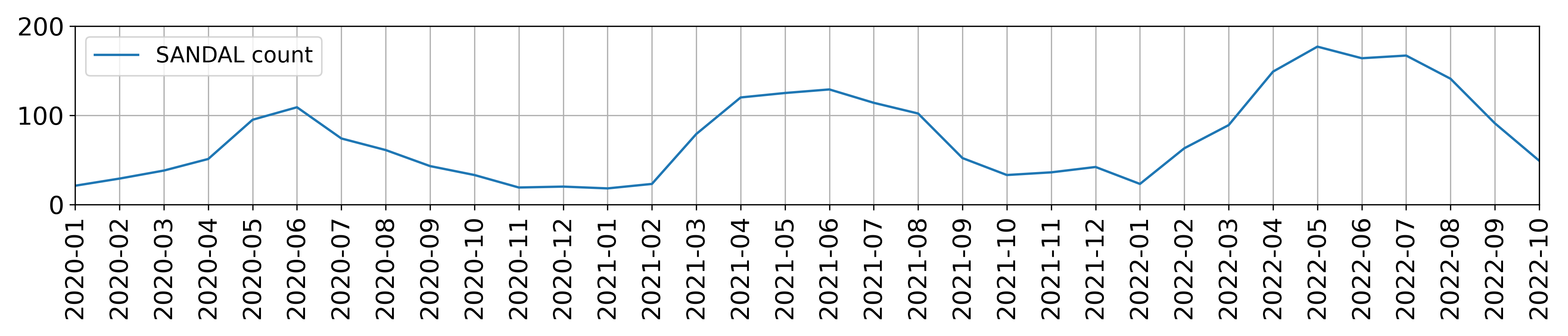
For each of the following regression models, use the visualizations shown above to select the value that is closest to the fitted model weights. If it is not possible to determine the model weight, select “Not enough info”. For the models below:

• The notation \text{boot} refers to the number of boots sold.
• The notation \text{sandal} refers to the number of sandals sold.
• \text{summer}=1 is a column with value 1 if the month is between March (03) and August (08), inclusive.
• \text{winter}=1 is a column with value 1 if the month is between September (09) and February (02), inclusive.

Problem 2.1

\text{predicted boot}_i = w_0

w_0:

• 0

• 50

• 100

• Not enough info

Problem 2.2

\text{predicted boot}_i = w_0 + w_1 \cdot \text{sandals}_i

w_0:

• -100

• -1

• 0

• 1

• 100

• Not enough info

w_1:

• -100

• -1

• 1

• 100

• Not enough info

Problem 2.3

\text{predicted boot}_i = w_0 + w_1 \cdot (\text{summer=1})_i

w_0:

• -100

• -1

• 0

• 1

• 100

• Not enough info

w_1:

• -80

• -1

• 0

• 1

• 80

• Not enough info

Problem 2.4

\text{predicted sandal}_i = w_0 + w_1 \cdot (\text{summer=1})_i

w_0:

• -20

• -1

• 0

• 1

• 20

• Not enough info

w_1:

• -80

• -1

• 0

• 1

• 80

• Not enough info

Problem 2.5

\text{predicted sandal}_i = w_0 + w_1 \cdot (\text{summer=1})_i + w_2 \cdot (\text{winter=1})_i

w_0:

• -20

• -1

• 0

• 1

• 20

• Not enough info

w_1:

• -80

• -1

• 0

• 1

• 80

• Not enough info

w_2:

• -80

• -1

• 0

• 1

• 80

• Not enough info

Problem 3

We will aim to build a classifier that takes in demographic information about a state from a particular year and predicts whether or not the state’s mean math score is higher than its mean verbal score that year.

In honor of the rotisserie chicken event on UCSD’s campus in March of 2023, sklearn released a new classifier class called ChickenClassifier.

Problem 3.1

ChickenClassifiers have many hyperparameters, one of which is height. As we increase the value of height, the model variance of the resulting ChickenClassifier also increases.

First, we consider the training and testing accuracy of a ChickenClassifier trained using various values of height. Consider the plot below.

• Note that accuracy is a metric that measures how well a classifier performs by comparing the number of correct predictions to the total number of predictions.

Which of the following depicts training accuracy vs. height?

• Option 1

• Option 2

• Option 3

Which of the following depicts testing accuracy vs. height?

• Option 1

• Option 2

• Option 3

ChickenClassifiers have another hyperparameter, color, for which there are four possible values: "yellow", "brown", "red", and "orange". To find the optimal value of color, we perform k-fold cross-validation with k=4. The results are given in the table below.

Problem 3.2

Which value of color has the best average validation accuracy?

• "yellow"

• "brown"

• "red"

• "orange"

Problem 3.3

True or False: It is possible for a hyperparameter value to have the best average validation accuracy across all folds, but not have the best validation accuracy in any one particular fold.

• True

• False

Problem 3.4

Now, instead of finding the best height and best color individually, we decide to perform a grid search that uses k-fold cross-validation to find the combination of height and color with the best average validation accuracy.

For the purposes of this question, assume that:

• We are performing k-fold cross validation.
• Our training set contains n rows, where n is greater than 5 and is a multiple of k.
• There are h_1 possible values of height and h_2 possible values of color.

Consider the following three subparts:

• A. What is the size of each fold?
• B. How many times is row 5 in the training set used for training?
• C. How many times is row 5 in the training set used for validation?

Choose from the following options.

• k

• \frac{k}{n}

• \frac{n}{k}

• \frac{n}{k} \cdot (k - 1)

• h_1h_2k

• h_1h_2(k-1)

• \frac{nh_1h_2}{k}

• None of the above

Problem 4

Consider the least squares regression model, \vec{h} = X \vec{w}. Assume that X and \vec{h} refer to the design matrix and hypothesis vector for our training data, and \vec y is the true observation vector.

Let \vec{w}_\text{OLS}^* be the parameter vector that minimizes mean squared error without regularization. Specifically:

\vec{w}_\text{OLS}^* = \arg\underset{\vec{w}}{\min} \frac{1}{n} \| \vec{y} - X \vec{w} \|^2_2

Let \vec{w}_\text{ridge}^* be the parameter vector that minimizes mean squared error with L_2 regularization, using a non-negative regularization hyperparameter \lambda (i.e. ridge regression). Specifically:

\vec{w}_\text{ridge}^* = \arg\underset{\vec{w}}{\min} \frac{1}{n} \| \vec y - X \vec{w} \|^2_2 + \lambda \sum_{j=1}^{p} w_j^2

For each of the following problems, fill in the blank.

Problem 4.1

If we set \lambda = 0, then \Vert \vec{w}_\text{OLS}^* \Vert^2_2 is ____ \Vert \vec{w}_\text{ridge}^* \Vert^2_2

• less than

• equal to

• greater than

• impossible to tell

Problem 4.2

For each of the remaining parts, you can assume that \lambda is set such that the predicted response vectors for our two models (\vec{h} = X \vec{w}_\text{OLS}^* and \vec{h} = X \vec{w}_\text{ridge}^*) is different.

The training MSE of the model \vec{h} = X \vec{w}_\text{OLS}^* is ____ than the model \vec{h} = X \vec{w}_\text{ridge}^*.

• less than

• equal to

• greater than

• impossible to tell

Problem 4.3

Now, assume we’ve fit both models using our training data, and evaluate both models on some unseen testing data.

The test MSE of the model \vec{h} = X \vec{w}_\text{OLS}^* is ____ than the model \vec{h} = X \vec{w}_\text{ridge}^*.

• less than

• equal to

• greater than

• impossible to tell

Problem 4.4

Assume that our design matrix X contains a column of all ones. The sum of the residuals of our model \vec{h} = X \vec{w}_\text{ridge}^* ____.

• equal to 0

• not necessarily equal to 0

Problem 4.5

As we increase \lambda, the bias of the model \vec{h} = X \vec{w}_\text{ridge}^* tends to ____.

• increase

• stay the same

• decrease

Problem 4.6

As we increase \lambda, the model variance of the model \vec{h} = X \vec{w}_\text{ridge}^* tends to ____.

• increase

• stay the same

• decrease

Problem 4.7

As we increase \lambda, the observation variance of the model \vec{h} = X \vec{w}_\text{ridge}^* tends to ____.

• increase

• stay the same

• decrease

Problem 5

Suppose we’d like to use gradient descent to minimize the function f(x) = x^3 + x^2. Suppose we choose a learning rate of \alpha = \frac{1}{4}.

Problem 5.1

Suppose x^{(t)} is our guess of the minimizing input x^{*} at timestep t, i.e. x^{(t)} is the result of performing t iterations of gradient descent, given some initial guess. Write an expression for x^{(t+1)}. Your answer should be an expression involving x^{(t)} and some constants.

Problem 5.2

Suppose x^{(0)} = -1.

• What is the value of x^{(1)}?

• Will gradient descent eventually converge, given the initial guess x^{(0)} = -1 and step size \alpha = \frac{1}{4}?

Problem 5.3

Suppose x^{(0)} = 1.

• What is the value of x^{(1)}?

• Will gradient descent eventually converge, given the initial guess x^{(0)} = 1 and step size \alpha = \frac{1}{4}?

Problem 6

For a given classifier, suppose the first 10 predictions of our classifier and 10 true observations are as follows: \begin{array}{|c|c|c|c|c|c|c|c|c|c|c|} \hline \textbf{Predictions} & 1 & 1 & 1 & 1 & 1 & 0 & 1 & 1 & 1 & 1 \\ \hline \textbf{True Label} & 0 & 1 & 1 & 1 & 0 & 0 & 0 & 1 & 1 & 1 \\ \hline \end{array}

1. What is the accuracy of our classifier on these 10 predictions?

2. What is the precision on these 10 predictions?

3. What is the recall on these 10 predictions?

Problem 7

Suppose we want to use logistic regression to classify whether a person survived the sinking of the Titanic. The first 5 rows of our dataset are given below.

\begin{array}{|c|c|c|c|} \hline & \textbf{Age} & \textbf{Survived} & \textbf{Female} \\ \hline 0 & 22.0 & 0 & 0 \\ \hline 1 & 38.0 & 1 & 1 \\ \hline 2 & 26.0 & 1 & 1 \\ \hline 3 & 35.0 & 1 & 1 \\ \hline 4 & 35.0 & 0 & 0 \\ \hline \end{array}

Suppose after training our logistic regression model we get \vec{w}^* = \begin{bmatrix} -1.2 \\ -0.005 \\ 2.5 \end{bmatrix}, where -1.2 is an intercept term, -0.005 is the optimal parameter corresponding to passenger’s age, and 2.5 is the optimal parameter corresponding to sex (1 if female, 0 otherwise).

Problem 7.1

Consider Sı̄lānah Iskandar Nāsı̄f Abı̄ Dāghir Yazbak, a 20 year old female. What chance did she have to survive the sinking of the Titanic according to our model? Give your answer as a probability in terms of \sigma. If there is not enough information, write “not enough information.”

Problem 7.2

Sı̄lānah Iskandar Nāsı̄f Abı̄ Dāghir Yazbak actually survived. What is the cross-entropy loss for our prediction in the previous part?

Problem 7.3

At what age would we predict that a female passenger is more likely to have survived the Titanic than not? In other words, at what age is the probability of survival for a female passenger greater than 0.5?

Hint: Since \sigma(0) = 0.5, we have that \sigma \left( \vec{w}^* \cdot \text{Aug}(\vec x_i) \right) = 0.5 \implies \vec{w}^* \cdot \text{Aug}(\vec x_i) = 0.

Problem 7.4

Let m be the odds of a given non-female passenger’s survival according to our logistic regression model, i.e., if the passenger had an 80% chance of survival, m would be 4, since their odds of survival are \frac{0.8}{0.2} = 4.

It turns out we can compute f, the odds of survival for a female passenger of the same age, in terms of m. Give an expression for f in terms of m.

Problem 8

Consider the following dataset of n=7 points in d=2 dimensions.

Problem 8.1

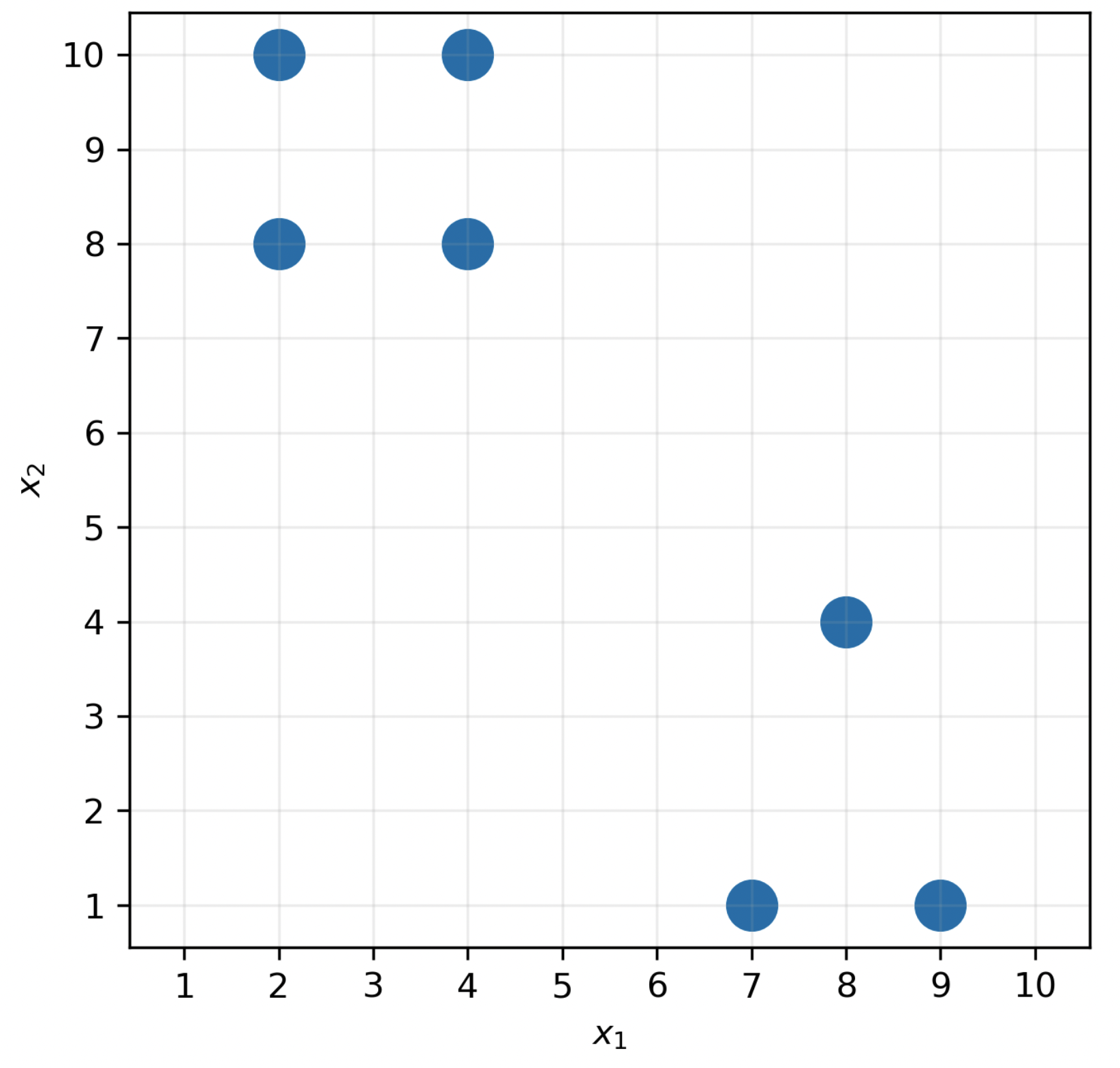
Suppose we decide to use agglomerative clustering to cluster the data. How many possible pairs of clusters could we combine in the first iteration?

Problem 8.2

Suppose we want to identify k=2 clusters in this dataset using k-means clustering.

Determine the centroids \vec{\mu}_1 and \vec{\mu}_2 that minimize inertia. (Let \vec{\mu}_1 be the centroid with a smaller x_1 coordinate.) Justify your answers.

Note: You don’t have to run the k-Means Clustering algorithm to answer this question.

Problem 8.3

What is the total inertia for the centroids you chose in the previous part? Show your work.

👋 Feedback: Find an error? Still confused? Have a suggestion? Let us know here.