← return to study.practicaldsc.org
Instructor(s): Suraj Rampure
This exam was administered in-person. The exam was closed-notes,
except students were allowed to bring two double-sided notes sheets. No
calculators were allowed. Students had 120 minutes to take this exam.
Access the original exam PDF
here.
Note: The Fall 2024 Final Exam was cumulative, but the
Spring 2025 Final Exam will not be cumulative.
As it gets colder outside, it’s important to make sure we’re taking
care of our skin! In this exam, we’ll work with the DataFrame
skin, which contains information about various skincare
products for sale at Sephora, a popular retailer that sells skincare
products. The first few rows of skin are shown below, but
skin has many more rows than are shown.
The columns in skin are as follows:
"Type" (str): The type of product. There are six
different possible types, three of which are shown above.
"Brand" (str): The brand of the product. As shown
above, brands can have multiple products.
"Name" (str): The name of product. Assume that
product names are unique.
"Price" (int): The price of the product, in a whole
number of dollars.
"Rating" (float): The rating of the product on
sephora.com; ranges from 0.0 to 5.0.
"Num Ingredients" (int): The number of ingredients
in the product.
"Sensitive" (int): 1 if the product is made for
individuals with sensitive skin, and 0 otherwise.
Throughout the exam, assume we have already run all necessary import statements.
An expensive product is one that costs at least $100.
Write an expression that evaluates to the proportion
of products in skin that are expensive.
Answer:
np.mean(skin['Price'] >= 100) or equivalent expressions
such as skin['Price'].ge(100).mean() or
(skin['Price'] >= 100).sum() / skin.shape[0].
To calculate the proportion of products in skin that are
expensive (price at least 100), we first evaluate the condition
skin['Price'] >= 100. This generates a Boolean series
where:
Each True represents a product with a price greater
than or equal to 100.
Each False represents a product with a price below
100.
When we call np.mean on this Boolean series, Python
internally treats True as 1 and False as 0.
The mean of this series therefore gives the proportion of
True values, which corresponds to the proportion of
products that meet the “expensive” criteria.
Alternatively, we can:
(skin['Price'] >= 100).sum().skin.shape[0]).Both approaches yield the same result.
The average score on this problem was 90%.
Fill in the blanks so that the expression below evaluates to the number of brands that sell fewer than 5 expensive products.
skin.groupby(__(i)__).__(ii)__(__(iii)__)["Brand"].nunique()(i):
"Brand"
"Name"
"Price"
["Brand", "Price"]
(ii):
agg
count
filter
value_counts
(iii): (Free response)
Answer:
(i): "Brand"(ii): filter(iii):
lambda x: (x['Price'] >= 100).sum() < 5The expression filters the grouped DataFrame to include only groups where the number of expensive products (those costing at least $100) is fewer than 5. Here’s how the expression works:
groupby('Brand'): Groups the
skin DataFrame by the unique values in the
"Brand" column, creating subgroups for each brand. Now,
when we apply the next step, it will perform the action on each
Brand group.filter: We use
filter instead of
agg (or other options) because
filter is designed to evaluate a condition
on the entire group and decide whether to include or exclude the group
in the final result. In this case, we want to include only groups
(brands) where the number of expensive products is fewer than 5.(lambda x: (x['Price'] >= 100).sum() < 5):
This lambda function runs on each group (in this case,
x is a DataFrame). It calculates the number of products in the group
where the price is greater than or equal to $100 (i.e., expensive
products). If this count is less than 5, the group is kept. Otherwise,
the group is excluded from our final result.Since we have an .nunique() at the end of our original
expression, we will return the number (n
in nunique) of unique brands.
Alternative forms for (iii) include:
- lambda x: np.sum(x['Price'] >= 100) < 5
- lambda x: x[x['Price'] >= 100].shape[0] < 5
- lambda x: x[x['Price'] >= 100].count() < 5
The average score on this problem was 72%.
This question is not in scope for Winter 2025.
Fill in each blank with one word to complete the sentence below.
The SQL keyword for filtering after grouping is __(i)__, and the SQL keyword for querying is __(ii)__.
Answer:
(i): HAVING
(ii): WHERE
An important distinction to make for part (ii) is that
we’re asking about the keyword for querying.
SELECT is incorrect, as SELECT is for
specifying a subset of columns, whereas querying is for
specifying a subset of rows.
The average score on this problem was 81%.
Consider the Series small_prices and vc,
both of which are defined below.
    small_prices = pd.Series([36, 36, 18, 100, 18, 36, 1, 1, 1, 36])

    vc = small_prices.value_counts().sort_values(ascending=False)
In each of the parts below, select the value that the provided expression evaluates to. If the expression errors, select “Error”.
vc.iloc[0]
0
1
2
3
4
18
36
100
Error
None of these
Answer: 4
vc computes the frequency of each value in small_prices,
sorts the counts in descending order, and stores the result in vc. The
resulting vc will look like this, where 36, 1, 18, and 100 are the
indices and 4, 3, 2, and 1 are the values:
iloc[0] retrieves the value at
integer position 0 in vc. The result is
4.
The average score on this problem was 73%.
vc.loc[0]
0
1
2
3
4
18
36
100
Error
None of these
Answer: Error
loc[0] attempts to retrieve the value
associated with the index 0 in vc.vc has indices 36, 1, 18, 10, and 0 is not a
valid index, this operation results in an error.
The average score on this problem was 83%.
vc.index[0]
0
1
2
3
4
18
36
100
Error
None of these
Answer: 36
index[0] retrieves the first index in
vc, which corresponds to the value 36.
The average score on this problem was 69%.
vc.iloc[1]
0
1
2
3
4
18
36
100
Error
None of these
Answer: 3
iloc[1] retrieves the value at
integer position 1 in vc, which is 3.
The average score on this problem was 74%.
vc.loc[1]
0
1
2
3
4
18
36
100
Error
None of these
Answer: 3
loc[1] retrieves the value associated
with the index 1 in vc, which corresponds
to the frequency of the value 1 in small_prices. The result
is 3.
The average score on this problem was 80%.
vc.index[1]
0
1
2
3
4
18
36
100
Error
None of these
Answer: 1
index[1] retrieves the positionally second index in
vc. The result is 1.
The average score on this problem was 64%.
Consider the DataFrames type_pivot,
clinique, fresh, and boscia,
defined below.
    type_pivot = skin.pivot_table(index="Type",
                                  columns="Brand",
                                  values="Sensitive",
                                  aggfunc=lambda s: s.shape[0] + 1)

    clinique = skin[skin["Brand"] == "clinique"]
    fresh = skin[skin["Brand"] == "fresh"]
    boscia = skin[skin["Brand"] == "BOSCIA"]
Three columns of type_pivot are shown below in
their entirety.
In each of the parts below, give your answer as an integer.
How many rows are in the following DataFrame?
clinique.merge(fresh, on="Type", how="inner")Answer: 10
The expression
clinique.merge(fresh, on="Type", how="inner") performs an
inner join on the "Type" column between
the clinique and fresh DataFrames. An inner
join includes only rows where the "Type" values are present
in both DataFrames.
From the provided type_pivot table, we know that the
overlapping ”Type” values between clinique and fresh
are:
Face Mask (3.0 for clinique, 4.0 for
fresh)
Moisturizer (3.0 for clinique, 3.0 for
fresh)
However, we must notice that the aggfunc for our
original pivot table is lambda s: s.shape[0] + 1. Thus, we
know that the values in the pivot table include an additional count of 1
for each group. This means the raw counts are actually:
Face Mask: 2 rows in clinique, 3 rows in
fresh
Moisturizer: 2 rows in clinique, 2 rows in
fresh
The inner join will match these rows based on "Type".
Since there are 2 rows in clinique for both Face Mask and
Moisturizer, and 3 and 2 rows in fresh respectively, the
result will have:
Face Mask: 2 (from clinique) × 3 (from
fresh) = 6 rows
Moisturizer: 2 (from clinique) × 2 (from
fresh) = 4 rows
The total number of rows in the resulting DataFrame is 6 + 4 = 10.
The average score on this problem was 42%.
How many rows are in the following DataFrame?
    (clinique.merge(fresh, on="Type", how="outer")
.merge(boscia, on="Type", how="outer"))Answer: 31
An outer join includes all rows from all DataFrames,
filling in missing values (NaN) for any Type
not present in one of them. From the table, the counts are calculated as
follows:
Remember that our pivot_table aggfunc is calculating
lambda s: s.shape[0] + 1 (so we need to subtract one from
the pivot table entry to get the actual number of rows).
cliniqueBOSCIAcliniqueBOSCIAcliniquefreshBOSCIAcliniquefreshcliniqueFinal Calculation: 5 \cdot 1 + 3 \cdot 1 + 2 \cdot 3 \cdot 3 + 2 \cdot 2 + 1 = 31
The average score on this problem was 27%.
Consider a sample of 60 skincare products. The name of one product from the sample is given below:
“our drops cream is the best drops drops for eye drops drops proven formula..."
The total number of terms in the product name above is unknown, but we know that the term drops only appears in the name 5 times.
Suppose the TF-IDF of drops in the product name above is \frac{2}{3}. Which of the following statements are NOT possible, assuming we use a base-2 logarithm? Select all that apply.
All 60 product names contain the term drops, including the one above.
14 other product names contain the term drops, in addition to the one above.
None of the 59 other product names contain the term drops.
There are 15 terms in the product name above in total.
There are 25 terms in the product name above in total.
Answer:
The TF-IDF score of a term is calculated as: \text{tf-idf}(t,d) = \text{tf}(t,d) \cdot \text{idf}(t) = \frac{\# \text{ of occurrences of } t \text{ in } d }{\text{total } \# \text{ of terms in } d} \cdot \log_2\left(\frac{\text{total } \# \text{ of documents}}{\# \text{ of documents in which } t \text{ appears}}\right)
We know:
t appears 5 times in d
Total number of documents = 60
\text{TF-IDF} = \frac{2}{3}
Let T be the total number of terms in d (d refers to the sentence at the top) and n refer to number of documents in which t appears, then substituting this into our formula gives us: \frac{5}{T} \cdot \log_2\left(\frac{60}{n}\right) = \frac{2}{3}
The problem then boils down to checking whether the above equation holds true in each of the five options
Option 1: All 60 product names contain the term drops.
This is NOT possible.
Option 2: 14 other product names contain the term drops.
This is possible.
Option 3: None of the 59 other product names contain the term drops.
This is NOT possible.
Option 4: There are 15 terms in the product name above in total. If T = 15, substituting into the TF equation, we get:
\text{TF} = \frac{5}{15} = \frac{1}{3}
\frac{1}{3} \cdot \text{IDF} = \frac{2}{3} \implies \text{IDF} = 2
Substituting \text{IDF} = 2 into the IDF formula:
2 = \log_2\left(\frac{60}{n}\right) 2 = \log_2(4) \implies \frac{60}{n} = 4 \implies n = 15
This is consistent with the problem’s constraints.
This is possible.
Option 5: There are 25 terms in the product name above in total. If T = 25, substituting into the TF equation: \text{TF} = \frac{5}{25} = \frac{1}{5} Substituting \text{TF} = \frac{1}{5} into the TF-IDF equation: \frac{1}{5} \cdot \text{IDF} = \frac{2}{3} \implies \text{IDF} = \frac{10}{3} Substituting \text{IDF} = \frac{10}{3} into the IDF formula: \frac{10}{3} = \log_2\left(\frac{60}{n}\right) This results in a value for n that is not an integer.
This is NOT possible.
The average score on this problem was 80%.
Suppose soup is a BeautifulSoup object representing the
homepage of a Sephora competitor.
Furthermore, suppose prods, defined below, is a list of
strings containing the name of every product on the site.
prods = [row.get("prod") for row in soup.find_all("row", class_="thing")]Given that prods[1] evaluates to
"Cleansifier", which of the following options describes the
source code of the site?
Option 1:
<row class="thing">prod: Facial Treatment Essence</row>
<row class="thing">prod: Cleansifier</row>
<row class="thing">prod: Self Tan Dry Oil SPF 50</row>
...
Option 2:
<row class="thing" prod="Facial Treatment Essence"></row>
<row class="thing" prod="Cleansifier"></row>
<row class="thing" prod="Self Tan Dry Oil SPF 50"></row>
...
Option 3:
<row prod="thing" class="Facial Treatment Essence"></row>
<row prod="thing" class="Cleansifier"></row>
<row prod="thing" class="Self Tan Dry Oil SPF 50"></row>
...
Option 4:
<row class="thing">prod="Facial Treatment Essence"</row>
<row class="thing">prod="Cleansifier"</row>
<row class="thing">prod="Self Tan Dry Oil SPF 50"</row>
...
Option 1
Option 2
Option 3
Option 4
Answer: Option 2
The given code:
prods = [row.get("prod") for row in soup.find_all("row", class_="thing")]retrieves all <row> elements with the class
"thing" and extracts the value of the "prod"
attribute for each.
Option 1:
In this structure, the product names appear as text content within the
<row> tags, not as an attribute.
row.get("prod") would return None.
Option 2:
Here, the product names are stored as the value of the
"prod" attribute. row.get("prod") successfully
retrieves these values.
Option 3:
In this structure, the "prod" attribute contains the value
"thing", and the product names are stored as the value of
the "class" attribute.
soup.find_all("row", class_="thing") will not retrieve any
of these tags since there are no tags with
class="thing".
Option 4:
In this structure, the product names are part of the text content inside
the <row> tags. row.get("prod") would
return None.
The average score on this problem was 76%.
Consider a dataset of n values, y_1, y_2, ..., y_n, all of which are positive. We want to fit a constant model, H(x) = h, to the data.
Let h_p^* be the optimal constant prediction that minimizes average degree-p loss, R_p(h), defined below.
R_p(h) = \frac{1}{n} \sum_{i = 1}^n | y_i - h |^p
For example, h_2^* is the optimal constant prediction that minimizes \displaystyle R_2(h) = \frac{1}{n} \sum_{i = 1}^n |y_i - h|^2.
In each of the parts below, determine the value of the quantity provided. By “the data", we are referring to y_1, y_2, ..., y_n.
h_0^*
The standard deviation of the data
The variance of the data
The mean of the data
The median of the data
The midrange of the data, \frac{y_\text{min} + y_\text{max}}{2}
The mode of the data
None of the above
Answer: The mode of the data
R_0(h) counts the number of incorrect predictions for each prediction, so choosing the most frequent value (mode) minimizes this count.
Note: This was our intended answer, as the idea here was to mirror 0-1 loss from discussion (and briefly mentioned in lecture). 0-1 loss is defined as:
L_{0-1}(y_i, h) = \begin{cases} 0 & \text{if } y_i = h \\ 1 & \text{if } y_i \neq h \end{cases}
But, we posed the question in a way that’s a little too vague, as 0^0 is undefined, and we need it to be 0 for this interpretation to hold. So, we gave everyone credit for this part.
The average score on this problem was 100%.
h_1^*
The standard deviation of the data
The variance of the data
The mean of the data
The median of the data
The midrange of the data, \frac{y_\text{min} + y_\text{max}}{2}
The mode of the data
None of the above
Answer: The median of the data
As seen in lecture, the minimizer of empirical risk for the constant model when using absolute loss is the median.
The average score on this problem was 87%.
R_1(h_1^*)
The standard deviation of the data
The variance of the data
The mean of the data
The median of the data
The midrange of the data, \frac{y_\text{min} + y_\text{max}}{2}
The mode of the data
None of the above
Answer: None of the above
As we discussed in the previous subpart, h_1^*, the minimizer of mean absolute error, is the median. So, R_1(h_1^*) is the mean absolute difference (or deviation) between all values and the median. This is not any of the answer choices, and in general, is not a quantity we studied in detail in class.
R_1(h_1^*) represents the sum of absolute deviations from the median divided by n:
R_1(h_1^*) = \frac{1}{n} \sum_{i=1}^n |y_i - h_1^*|
The average score on this problem was 44%.
h_2^*
The standard deviation of the data
The variance of the data
The mean of the data
The median of the data
The midrange of the data, \frac{y_\text{min} + y_\text{max}}{2}
The mode of the data
None of the above
Answer: The mean of the data
The minimizer of empirical risk for the constant model when using squared loss is the mean.
The average score on this problem was 81%.
R_2(h_2^*)
The standard deviation of the data
The variance of the data
The mean of the data
The median of the data
The midrange of the data, \frac{y_\text{min} + y_\text{max}}{2}
The mode of the data
None of the above
Answer: The variance of the data
R_2(h) represents the mean squared error of the constant prediction, h. In the previous part, we discussed that h_2^*, the minimizer of R_2(h), is the mean, \bar{y}. So, R_2(h_2^*) is then:
R_2(h_2^*) = \frac{1}{n} \sum_{i = 1}^n (y_i - h_2^*)^2 = \frac{1}{n} \sum_{i = 1}^n (y_i - \bar{y})^2
This is the definition of the variance of y.
The average score on this problem was 70%.
Now, suppose we want to find the optimal constant prediction, h_\text{U}^*, using the “Ulta" loss function, defined below.
L_U(y_i, h) = y_i (y_i - h)^2
To find h_\text{U}^*, suppose we minimize average Ulta loss (with no regularization). How does h_\text{U}^* compare to the mean of the data, M?
h_\text{U}^* > M
h_\text{U}^* \geq M
h_\text{U}^* = M
h_\text{U}^* \leq M
h_\text{U}^* < M
Answer: h_\text{U}^* \geq M
Minimizing the average Ulta loss means minimizing the empirical risk:
R_U(h) = \frac{1}{n} \sum_{i = 1}^n y_i (y_i - h)^2.
This resembles minimizing mean squared error, except each y_i is given a weight of y_i. Since larger y_i values contribute more to the loss, the minimizer is pulled toward higher values to reduce their impact. This results in h_\text{U}^* being greater than the mean of the data.
The average score on this problem was 42%.
Now, to find the optimal constant prediction, we will instead minimize regularized average Ulta loss, R_\lambda(h), where \lambda is a non-negative regularization hyperparameter:
R_\lambda(h) = \left( \frac{1}{n} \sum_{i = 1}^n y_i (y_i - h)^2 \right) + \lambda h^2
It can be shown that \displaystyle \frac{\partial R_\lambda(h)}{\partial h}, the derivative of R_\lambda(h) with respect to h, is:
\frac{\partial R_\lambda(h)}{\partial h} = -2 \left( \frac{1}{n} \sum_{i = 1}^n y_i (y_i - h) - \lambda h \right)
Find h^*, the constant prediction that minimizes R_\lambda(h). Show your work, and put a \boxed{\text{box}} around your final answer, which should be an expression in terms of y_i, n, and/or \lambda.
Answer: h^* = \frac{\sum_{i = 1}^n y_i^2}{\sum_{i = 1}^n y_i + n\lambda}
To minimize the regularized average Ulta loss, we solve for h by setting
\frac{\partial R_\lambda(h)}{\partial h} =
0.
Step 1: Compute the derivative and set it to zero
\frac{\partial R_\lambda(h)}{\partial h} = -2 \left( \frac{1}{n} \sum_{i = 1}^n y_i (y_i - h) \right) + 2\lambda h = 0
Step 2: Expand and simplify
\frac{1}{n} \sum_{i = 1}^n y_i^2 - \frac{1}{n} \sum_{i = 1}^n y_i h - \lambda h = 0
Rearrange terms:
\frac{1}{n} \sum_{i = 1}^n y_i^2 = h \left( \frac{1}{n} \sum_{i = 1}^n y_i + \lambda \right)
Step 3: Solve for h
Divide both sides by \frac{1}{n} \sum_{i = 1}^n y_i + \lambda:
h^* = \frac{\frac{1}{n} \sum_{i = 1}^n y_i^2}{\frac{1}{n} \sum_{i = 1}^n y_i + \lambda}
Step 4: Multiply by \frac{n}{n}
h^* = \frac{\sum_{i = 1}^n y_i^2}{\sum_{i = 1}^n y_i + n\lambda}
The average score on this problem was 71%.
Suppose we want to fit a simple linear regression model (using squared loss) that predicts the number of ingredients in a product given its price. We’re given that:
The average cost of a product in our dataset is $40, i.e. \bar x = 40.
The average number of ingredients in a product in our dataset is 15, i.e. \bar y = 15.
The intercept and slope of the regression line are w_0^* = 11 and w_1^* = \frac{1}{10}, respectively.
Suppose Victors’ Veil (a skincare product) costs $40 and has 11 ingredients. What is the squared loss of our model’s predicted number of ingredients for Victors’ Veil? Give your answer as a number.
Answer: 16
Using the equation of the regression model we have seen in
class:
H(x) = w_0^* + w_1^* x
Substitute w_0^* = 11, w_1^* = \frac{1}{10}, and x = 40:
H(40) = 11 + \frac{1}{10} \cdot 40 = 11 + 4
= 15
The squared loss is:
L = (y - H(x_i))^2
Substituting y = 11 (actual) and
H(x_i) = 15 (predicted):
L = (11 - 15)^2 = (-4)^2 = 16
The average score on this problem was 86%.
Is it possible to answer part (a) above just by knowing \bar x and \bar y, i.e. without knowing the values of w_0^* and w_1^*?
Yes; the values of w_0^* and w_1^* don’t impact the answer to part (a).
No; the values of w_0^* and w_1^* are necessary to answer part (a).
Answer: Yes; the values of w_0^* and w_1^* don’t impact the answer to part (a).
A fact from lecture is that the regression line always passes through the point (\bar{x}, \bar{y}), meaning that for an average x, we always predict an average y. We’re given that \bar{x} = 40 and \bar{y} = 15, meaning that for a product that costs $40 we will predict that it has 15 ingredients, no matter what the slope and intercept end up being.
The average score on this problem was 56%.
Suppose x_i represents the price of product i, and suppose u_i represents the negative price of product i. In other words, for i = 1, 2, ..., n, where n is the number of points in our dataset:
u_i = - x_i
Suppose U is the design matrix for the simple linear regression model that uses negative price to predict number of ingredients. Which of the following matrices could be U^TU?
\begin{bmatrix} -15 & 600 \\ 600 &
-30000 \end{bmatrix}
\begin{bmatrix} 15 & -600 \\ -600
& 30000 \end{bmatrix}
\begin{bmatrix} -15 & 450 \\ 450 &
-30000 \end{bmatrix}
\begin{bmatrix} 15 & -450 \\ -450
& 30000 \end{bmatrix}
Answer: \begin{bmatrix} 15 & -600 \\ -600 & 30000 \end{bmatrix}
The design matrix U is defined as: U = \begin{bmatrix} 1 & -x_1 \\ 1 & -x_2 \\ \vdots & \vdots \\ 1 & -x_n \end{bmatrix} where 1 represents the intercept term, and -x_i represents the negative price of product i. Thus:
U^T U = \begin{bmatrix} 1 & 1 & \cdots & 1 \\ -x_1 & -x_2 & \cdots & -x_n \end{bmatrix} \begin{bmatrix} 1 & -x_1 \\ 1 & -x_2 \\ \vdots & \vdots \\ 1 & -x_n \end{bmatrix}
When we multiply this out, we get: U^T U = \begin{bmatrix} n & -\sum_{i = 1}^n x_i \\ -\sum_{i = 1}^n x_i & \sum_{i = 1}^n x_i^2 \end{bmatrix}
Conceptually, this matrix represents:
\begin{bmatrix}
\text{Number of elements} & \text{Sum of the negative values of the
data} \\
\text{Sum of the negative values of the data} & \text{Sum of squared
values of the data}
\end{bmatrix}.
We know that the sum of all elements in a series is equal to the mean of the series multiplied by the number of elements in the series. \sum_{i = 1}^n x_i = n \cdot \bar{x}
\bar{x} is equal to 40. The first element in the matrix, 15, represents the number of elements in the
series. Thus,
\displaystyle \sum_{i = 1}^n x_i = 40 \cdot 15 = 600
and the solution must be as follows:
\begin{bmatrix} n & -\sum_{i = 1}^n x_i \\ -\sum_{i = 1}^n x_i & \sum_{i = 1}^n x_i^2 \end{bmatrix} = \begin{bmatrix} 15 & -600 \\ -600 & 30000 \end{bmatrix}
The average score on this problem was 74%.
Suppose we want to fit a multiple linear regression model (using squared loss) that predicts the number of ingredients in a product given its price and various other information.
From the Data Overview page, we know that there are 6 different types of products. Assume in this question that there are 20 different product brands. Consider the models defined in the table below.
| Model Name | Intercept | Price | Type | Brand |
|---|---|---|---|---|
| Model A | Yes | Yes | No | One hot encoded |
without drop="first" |
||||
| Model B | Yes | Yes | No | No |
| Model C | Yes | Yes | One hot encoded | |
without drop="first" |
||||
| Model D | No | Yes | One hot encoded | One hot encoded |
with drop="first" |
with drop="first" |
|||
| Model E | No | Yes | One hot encoded | One hot encoded |
with drop="first" |
without drop="first" |
For instance, Model A above includes an intercept term, price as a
feature, one hot encodes brand names, and doesn’t use
drop="first" as an argument to OneHotEncoder
in sklearn.
In parts 1 through 3, you are given a model. For each model provided, state the number of columns and the rank (i.e. number of linearly independent columns) of the design matrix, X. Some of part 1 is already done for you as an example.
Model A
Number of columns in X:
Rank of X: 21
Answer:
Number of columns in X: 22
Model A includes an intercept, the price feature, and a one-hot encoding of the 20 brands without dropping the first category. The intercept adds 1 column, the price adds 1 column, and the one-hot encoding for brands adds 20 columns. The rank is 21 because one of the brand categories can be predicted by the others (i.e., the columns are linearly dependent).
The rank is 21 because when encoding categorical variables (such as brands), dropping the first category avoids introducing perfect multicollinearity. By not dropping a category, we increase the rank by 1, but this still maintains linear dependence among the columns.
The average score on this problem was 80%.
Model B
Number of columns in X:
Rank of X:
Answer:
Number of columns in X:
2
Rank of X: 2
Model B includes an intercept and the price feature, but no one-hot encoding for the brands or product types. The intercept and price are linearly independent, resulting in both the number of columns and the rank being 2.
The average score on this problem was 82%.
Model C
Number of columns in X:
Rank of X:
Answer:
Number of columns in X:
8
Rank of X: 7
Model C includes an intercept, the price feature, and a one-hot encoding of the 6 product types without dropping the first category. The intercept adds 1 column, the price adds 1 column, and the one-hot encoding for the product types adds 6 columns. However, one column is linearly dependent because we didn’t drop one of the one-hot encoded columns, reducing the rank to 7.
This happens because if we have 6 product types, one of the columns can always be written as a linear combination of the other five. Thus, we lose one degree of freedom in the matrix, and the rank is 7.
The average score on this problem was 81%.
Which of the following models are NOT guaranteed to have residuals that sum to 0?
Hint: Remember, the residuals of a fit model are the differences between actual and predicted y-values, among the data points in the training set.
Model A
Model B
Model C
Model D
Model E
Answer: Model D
For residuals to sum to zero in a linear regression model, the design matrix must include either an intercept term (Models A - C) or equivalent redundancy in the encoded variables to act as a substitute for the intercept (Model E). Models that lack both an intercept and equivalent redundancy, such as Model D, are not guaranteed to have residuals sum to zero.
For a linear model, the residual vector \vec{e} is chosen such that it is orthogonal to the column space of the design matrix X. If one of the columns of X is a column of all ones (as in the case with an intercept term), it ensures that the sum of the residuals is zero. This is because the error vector \vec{e} is orthogonal to the span of X, and hence X^T \vec{e} = 0. If there isn’t a column of all ones, but we can create such a column using a linear combination of the other columns in X, the residuals will still sum to zero. Model D lacks this structure, so the residuals are not guaranteed to sum to zero.
In contrast, one-hot encoding without dropping any category can behave like an intercept because it introduces a column for each category, allowing the model to adjust its predictions as if it had an intercept term. The sum of the indicator variables in such a setup equals 1 for every row, creating a similar effect to an intercept, which is why residuals may sum to zero in these cases.
The average score on this problem was 60%.
Suppose we want to create polynomial features and use ridge regression (i.e. minimize mean squared error with L_2 regularization) to fit a linear model that predicts the number of ingredients in a product given its price.
To choose the polynomial degree and regularization hyperparameter, we
use cross-validation through GridSearchCV in
sklearn using the code below.
    searcher = GridSearchCV(
        make_pipeline(PolynomialFeatures(include_bias=False),
                      Ridge()),

        param_grid={"polynomialfeatures__degree": np.arange(1, D + 1),
                    "ridge__alpha": 2 ** np.arange(1, L + 1)},

        cv=K # K-fold cross-validation.
    )
    searcher.fit(X_train, y_train)
Assume that there are N rows in
X_train, where N is a
multiple of K (the number of folds used
for cross-validation).
In each of the parts below, give your answer as an expression involving D, L, K, and/or N. Part (a) is done for you as an example.
How many combinations of hyperparameters are being considered? Answer: LD
Answer: LD
There are L possible values of \lambda and D possible polynomial degrees, giving LD total combinations of hyperparameters.
Each time a model is trained, how many points are being used to train the model?
Answer: N \cdot \frac{K-1}{K}
In K-fold cross-validation, the data is split into K folds. Each time a model is trained, one fold is used for validation, and the remaining K-1 folds are used for training. Since N is evenly split among K folds, each fold contains \frac{N}{K} points. The training data, therefore, consists of N - \frac{N}{K} = N \cdot \frac{K-1}{K} points.
The average score on this problem was 72%.
In total, how many times are
X_train.iloc[1] and X_train.iloc[-1]
both used for training a model at the same
time? Assume that these two points are in different folds.
Answer: LD \times (K-2)
In K-fold cross-validation, X_train.iloc[1] and
X_train.iloc[-1] are in different folds and can only be
used together for training when neither of their respective folds is the
validation set. This happens in (K-2)
folds for each combination of polynomial degree (D) and regularization hyperparameter (L). Since there are L \times D total combinations in the grid
search, the two points are used together for training LD \times (K-2) times.
The average score on this problem was 53%.
Suppose we want to use LASSO (i.e. minimize mean squared error with L_1 regularization) to fit a linear model that predicts the number of ingredients in a product given its price and rating.
Let \lambda be a non-negative regularization hyperparameter. Using cross-validation, we determine the average validation mean squared error — which we’ll refer to as AVMSE in this question — for several different choices of \lambda. The results are given below.
As \lambda increases, what happens to model complexity and model variance?
Model complexity and model variance both increase.
Model complexity increases while model variance decreases.
Model complexity decreases while model variance increases.
Model complexity and model variance both decrease.
Answer: Model complexity and model variance both decrease.
As \lambda increases, the L_1 regularization penalizes larger coefficient values more heavily, forcing the model to forget the details in the training data and focus on the bigger picture. This effectively reduces the number of non-zero coefficients, decreasing model complexity. Since model complexity and model variance are the same thing, variance also decreases.
The average score on this problem was 64%.
What does the value A on the graph above correspond to?
The AVMSE of the \lambda we’d choose to use to train a model.
The AVMSE of an unregularized multiple linear regression model.
The AVMSE of the constant model.
Answer: The AVMSE of an unregularized multiple linear regression model.
Point A represents the case where \lambda = 0, meaning no regularization is applied. This corresponds to an unregularized multiple linear regression model.
The average score on this problem was 80%.
What does the value B on the graph above correspond to?
The AVMSE of the \lambda we’d choose to use to train a model.
The AVMSE of an unregularized multiple linear regression model.
The AVMSE of the constant model.
Answer: The AVMSE of the \lambda we’d choose to use to train a model.
Point B is the minimum point on the graph, indicating the optimal \lambda value that minimizes the AVMSE. This is because we don’t typically regularize the intercept term’s coefficient, w_0^*.
The average score on this problem was 91%.
What does the value C on the graph above correspond to?
The AVMSE of the \lambda we’d choose to use to train a model.
The AVMSE of an unregularized multiple linear regression model.
The AVMSE of the constant model.
Answer: The AVMSE of the constant model.
Point C represents the AVMSE when \lambda is very large, effectively forcing all coefficients to zero. This corresponds to the constant model.
The average score on this problem was 83%.
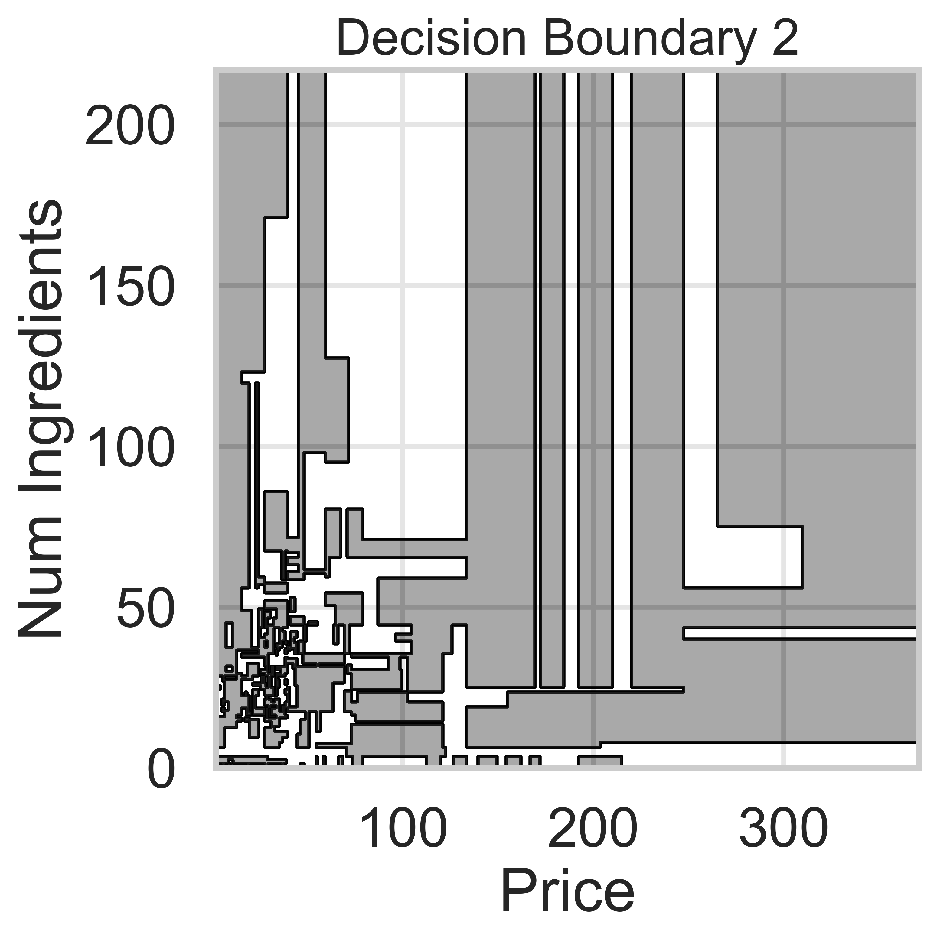
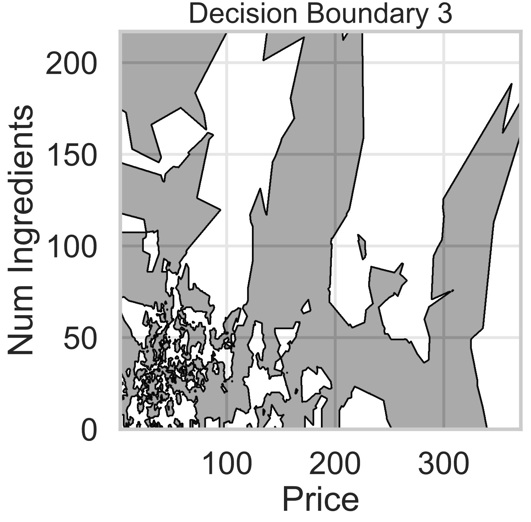
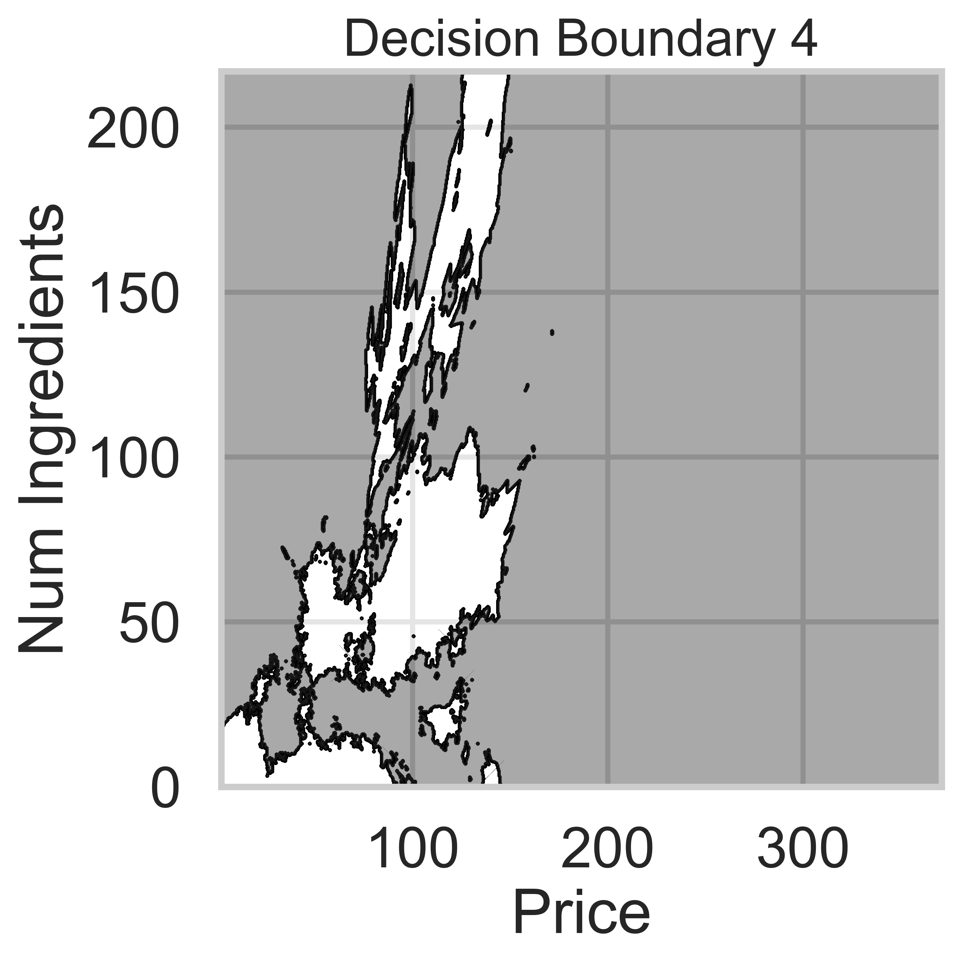
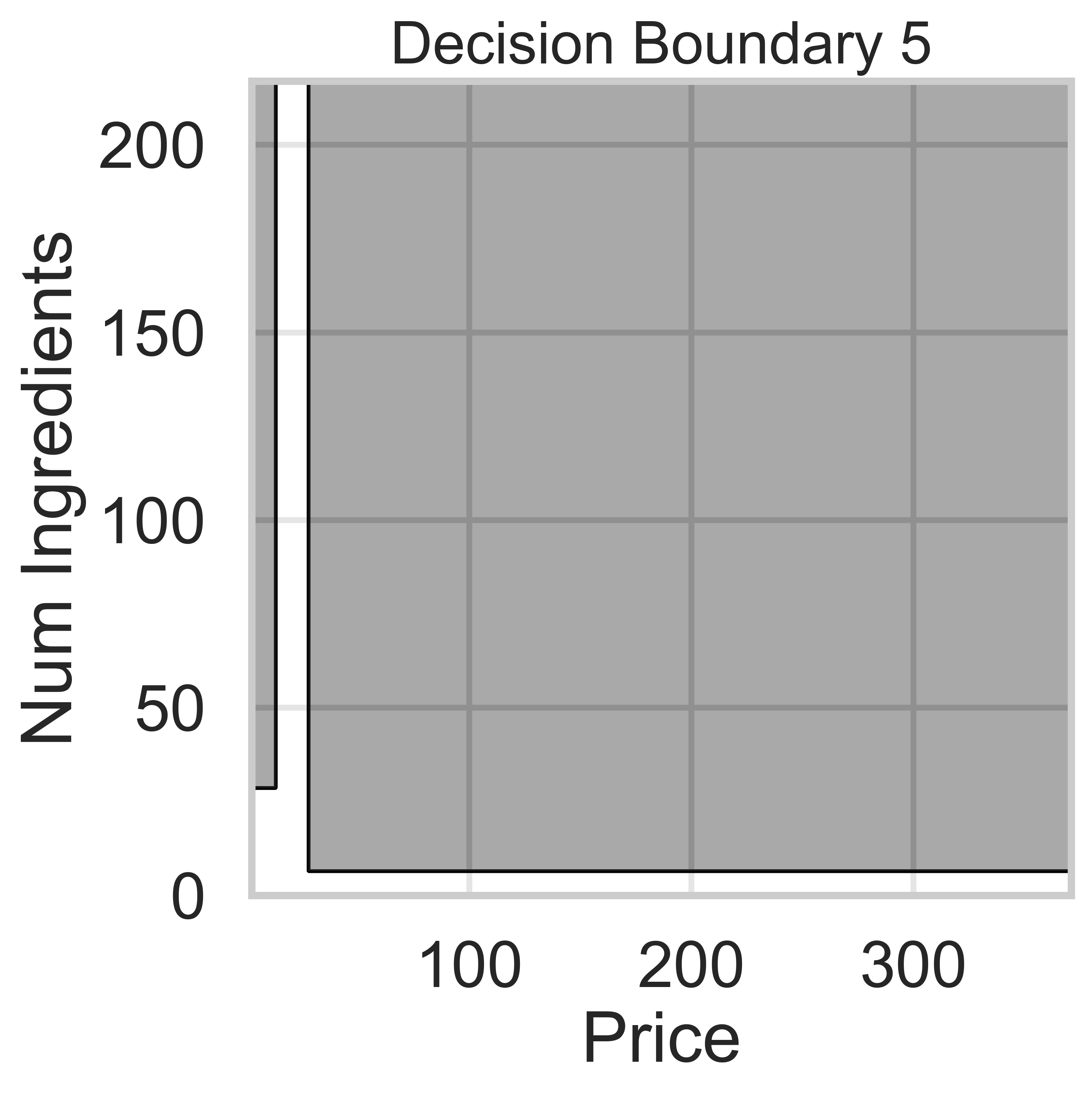
Suppose we fit five different classifiers that predict whether a product is designed for sensitive skin, given its price and number of ingredients. In the five decision boundaries below, the gray-shaded regions represent areas in which the classifier would predict that the product is designed for sensitive skin (i.e. predict class 1).
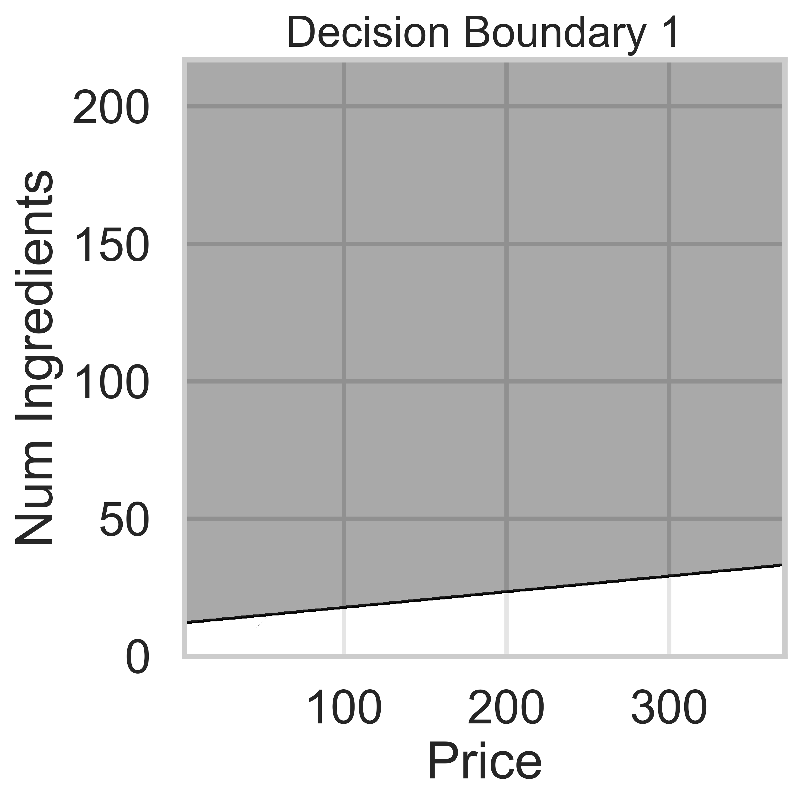
Which model does Decision Boundary 1 correspond to?
k-nearest neighbors with k = 3
k-nearest neighbors with k = 100
Decision tree with \text{max depth} = 3
Decision tree with \text{max depth} = 15
Logistic regression
Answer: Logistic regression
Logistic regression is a linear classification technique, meaning it creates a single linear decision boundary between classes. Among the five decision boundaries, only Decision Boundary 1 is linear, making it the correct answer.
The average score on this problem was 93%.
Which model does Decision Boundary 2 correspond to?
k-nearest neighbors with k = 3
k-nearest neighbors with k = 100
Decision tree with \text{max depth} = 3
Decision tree with \text{max depth} = 15
Logistic regression
Answer: Decision tree with \text{max depth} = 15
We know that Decision Boundaries 2 and 5 are decision trees, since the decision boundaries are parallel to the axes. Decision boundaries for decision trees are parallel to axes because the tree splits the feature space based on one feature at a time, creating partitions aligned with that feature’s axis (e.g., “Price ≤ 100” results in a vertical split).
Decision Boundary 2 is more complicated than Decision Boundary 5, so we can assume there are more levels.
The average score on this problem was 82%.
Which model does Decision Boundary 3 correspond to?
k-nearest neighbors with k = 3
k-nearest neighbors with k = 100
Decision tree with \text{max depth} = 3
Decision tree with \text{max depth} = 15
Logistic regression
Answer: k-nearest neighbors with k = 3
k-nearest neighbors decision boundaries don’t follow straight lines like logistic regression or decision trees. Thus, boundaries 3 and 4 are k-nearest neighbors.
A lower value of k means the model is more sensitive to local variations in the data. Since Decision Boundary 3 has more complex and irregular regions than Decision Boundary 4, it corresponds to k = 3, where the model closely follows the training data.
For example, if in our training data we had 3 points in the group represented by the light-shaded region at (300, 150), the decision boundary for k-nearest neighbors with k = 3 would be light-shaded at (300, 150), whereas it may be dark-shaded for k-nearest neighbors with k = 100.
The average score on this problem was 59%.
Which model does Decision Boundary 4 correspond to?
k-nearest neighbors with k = 3
k-nearest neighbors with k = 100
Decision tree with \text{max depth} = 3
Decision tree with \text{max depth} = 15
Logistic regression
Answer: k-nearest neighbors with k = 100
k-nearest neighbors decision boundaries don’t follow straight lines like logistic regression or decision trees. Thus, boundaries 3 and 4 are k-nearest neighbors.
k-nearest neighbors decision boundaries adapt to the training data, but increasing k makes the model less sensitive to local variations.
Since Decision Boundary 4 is smoother and has fewer regions than Decision Boundary 3, it corresponds to k = 100, where predictions are averaged over a larger number of neighbors, making the boundary less sensitive to individual data points.
The average score on this problem was 56%.
Suppose we fit a logistic regression model that predicts whether a product is designed for sensitive skin, given its price, x^{(1)}, number of ingredients, x^{(2)}, and rating, x^{(3)}. After minimizing average cross-entropy loss, the optimal parameter vector is as follows:
\vec{w}^* = \begin{bmatrix} -1 \\ 1 / 5 \\ - 3 / 5 \\ 0 \end{bmatrix}
In other words, the intercept term is -1, the coefficient on price is \frac{1}{5}, the coefficient on the number of ingredients is -\frac{3}{5}, and the coefficient on rating is 0.
Consider the following four products:
Wolfcare: Costs $15, made of 20 ingredients, 4.5 rating
Go Blue Glow: Costs $25, made of 5 ingredients, 4.9 rating
DataSPF: Costs $50, made of 15 ingredients, 3.6 rating
Maize Mist: Free, made of 1 ingredient, 5.0 rating
Which of the following products have a predicted probability of being designed for sensitive skin of at least 0.5 (50%)? For each product, select Yes or No.
Wolfcare:
Yes
No
Go Blue Glow:
Yes
No
DataSPF:
Yes
No
Maize Mist:
Yes
No
Using the sigmoid function, we can predict the probabliity using this general formula -
P(y = 1 | \vec{x}) = \sigma(\vec{w}^T \vec{x})
where \sigma(x) = \frac{1}{1 + e^{-x}} is the sigmoid function.
We calculate z = \vec{w}^T \vec{x} for each product and then apply the sigmoid function to find the probability P(y = 1 | \vec{x}). If the probability is greater than or equal to 0.5, the product is predicted to be designed for sensitive skin.
Wolfcare:
z = \begin{bmatrix} -1 \\ \frac{1}{5} \\ -\frac{3}{5} \\ 0 \end{bmatrix}^T \cdot \begin{bmatrix} 1 \\ 15 \\ 20 \\ 4.5 \end{bmatrix} z = -1 + \frac{1}{5}(15) - \frac{3}{5}(20) + 0 = -1 + 3 - 12 = -10 P = \frac{1}{1 + e^{-(-10)}} = \frac{1}{1 + e^{10}} \approx 0
Decision: No, as P < 0.5
Go Blue Glow:
z = \begin{bmatrix} -1 \\ \frac{1}{5} \\ -\frac{3}{5} \\ 0 \end{bmatrix}^T \cdot \begin{bmatrix} 1 \\ 25 \\ 5 \\ 4.9 \end{bmatrix} z = -1 + \frac{1}{5}(25) - \frac{3}{5}(5) + 0 = -1 + 5 - 3 = 1 P = \frac{1}{1 + e^{-1}} \approx \frac{1}{1 + 0.3679} \approx 0.73
Decision: Yes, as P \geq 0.5.
DataSPF:
z = \begin{bmatrix} -1 \\ \frac{1}{5} \\ -\frac{3}{5} \\ 0 \end{bmatrix}^T \cdot \begin{bmatrix} 1 \\ 50 \\ 15 \\ 3.6 \end{bmatrix} z = -1 + \frac{1}{5}(50) - \frac{3}{5}(15) + 0 = -1 + 10 - 9 = 0 P = \frac{1}{1 + e^{-0}} = \frac{1}{2} = 0.5
Decision: Yes, as P \geq 0.5.
Maize Mist: z = \begin{bmatrix} -1 \\ \frac{1}{5} \\ -\frac{3}{5} \\ 0 \end{bmatrix}^T \cdot \begin{bmatrix} 1 \\ 0 \\ 1 \\ 5.0 \end{bmatrix} z = -1 + \frac{1}{5}(0) - \frac{3}{5}(1) + 0 = -1 - 0.6 = -1.6 P = \frac{1}{1 + e^{-(-1.6)}} = \frac{1}{1 + e^{1.6}} \approx \frac{1}{1 + 4.953} \approx 0.17 Decision: No, as P < 0.5
The average score on this problem was 85%.
Suppose, again, that we fit a logistic regression model that predicts whether a product is designed for sensitive skin. We’re deciding between three thresholds, A, B, and C, all of which are real numbers between 0 and 1 (inclusive). If a product’s predicted probability of being designed for sensitive skin is above our chosen threshold, we predict they belong to class 1 (yes); otherwise, we predict class 0 (no).
The confusion matrices of our model on the test set for all three thresholds are shown below.
\begin{array}{ccc} \textbf{$A$} & \textbf{$B$} & \textbf{$C$} \\ \begin{array}{|l|c|c|} \hline & \text{Pred.} \: 0 & \text{Pred.} \: 1 \\ \hline \text{Actually} \: 0 & 40 & 5 \\ \hline \text{Actually} \: 1 & 35 & 35 \\ \hline \end{array} & \begin{array}{|l|c|c|} \hline & \text{Pred.} \: 0 & \text{Pred.} \: 1 \\ \hline \text{Actually} \: 0 & 5 & 40 \\ \hline \text{Actually} \: 1 & 10 & ??? \\ \hline \end{array} & \begin{array}{|l|c|c|} \hline & \text{Pred.} \: 0 & \text{Pred.} \: 1 \\ \hline \text{Actually} \: 0 & 10 & 35 \\ \hline \text{Actually} \: 1 & 30 & 40 \\ \hline \end{array} \end{array}
Suppose we choose threshold A, i.e. the leftmost confusion matrix. What is the precision of the resulting predictions? Give your answer as an unsimplified fraction.
Answer: \frac{35}{40}
The precision of a binary classification model is calculated as:
\text{Precision} = \frac{\text{True Positives (TP)}}{\text{True Positives (TP)} + \text{False Positives (FP)}}
From the confusion matrix for threshold A:
\begin{array}{|l|c|c|} \hline & \text{Pred.} \: 0 & \text{Pred.} \: 1 \\ \hline \text{Actually} \: 0 & 40 & 5 \\ \hline \text{Actually} \: 1 & 35 & 35 \\ \hline \end{array}
The number of true positives (TP) is 35, and the number of false positives (FP) is 5. Substituting into the formula:
\text{Precision} = \frac{35}{35 + 5} = \frac{35}{40}
The average score on this problem was 85%.
What is the missing value (???) in the confusion matrix for threshold B? Give your answer as an integer.
Answer: 60
From the confusion matrix for threshold B:
\begin{array}{|l|c|c|} \hline & \text{Pred.} \: 0 & \text{Pred.} \: 1 \\ \hline \text{Actually} \: 0 & 5 & 40 \\ \hline \text{Actually} \: 1 & 10 & ??? \\ \hline \end{array}
The sum of all entries in a confusion matrix must equal the total number of samples. For thresholds A and C, the total number of samples is:
40 + 5 + 35 + 35 = 115
Using this total, for threshold B, the entries provided are:
5 + 40 + 10 + ??? = 115
Solving for the missing value (???):
115 - (5 + 40 + 10) = 60
Thus, the missing value for threshold B is:
60
The average score on this problem was 90%.
Using the information in the three confusion matrices, arrange the thresholds from largest to smallest. Remember that 0 \leq A, B, C \leq 1.
A > B > C
A > C > B
B > A > C
B > C > A
C > A > B
C > B > A
Answer: A > C > B
Thresholds can be arranged based on their strictness. The higher a model’s threshold is, the fewer positive predictions and the more negative predictions it has. Model A made 40 negative predictions, Model B made 5 negative predictions and Model C made 10 negative predictions. Sorting these in descending order with more negative predictions implying a stricter threshold we get -
A > C > B
The average score on this problem was 67%.
Remember that in our classification problem, class 1 means the product is designed for sensitive skin, and class 0 means the product is not designed for sensitive skin. In one or two English sentences, explain which is worse in this context and why: a false positive or a false negative.
Answer: False positive
A false positive is worse, as it would mean we predict a product is safe when it isn’t; someone with sensitive skin may use it and it could harm them.
The average score on this problem was 91%.
Let \vec{x} = \begin{bmatrix} x_1 \\ x_2 \end{bmatrix}. Consider the function \displaystyle Q(\vec x) = x_1^2 - 2x_1x_2 + 3x_2^2 - 1.
Fill in the blank to complete the definition of \nabla Q(\vec x), the gradient of Q.
\nabla Q(\vec x) = \begin{bmatrix} 2(x_1 - x_2) \\ \\ \_\_\_\_ \end{bmatrix}
What goes in the blank? Show your work, and put a your final answer, which should be an expression involving x_1 and/or x_2.
Answer: -2x_1 + 6x_2
The gradient of Q(\vec{x}) is given by: \nabla Q(\vec{x}) = \begin{bmatrix} \frac{\partial Q}{\partial x_1} \\ \frac{\partial Q}{\partial x_2} \end{bmatrix}
First, calculate the partial derivative: Partial derivative with respect to x_1 is provided to us in the question: 2x_1 - 2x_2
Partial derivative with respect to x_2: \frac{\partial Q}{\partial x_2} = -2x_1 + 6x_2
Thus, the gradient is: \nabla Q(\vec{x}) = \begin{bmatrix} 2(x_1 - x_2) \\ -2x_1 + 6x_2 \end{bmatrix}
The average score on this problem was 87%.
We decide to use gradient descent to minimize Q, using an initial guess of \vec x^{(0)} = \begin{bmatrix} 1 \\ 1 \end{bmatrix} and a learning rate/step size of \alpha.
If after one iteration of gradient descent, we have \vec{x}^{(1)} = \begin{bmatrix} 1 \\ -4 \end{bmatrix}, what is \alpha?
\displaystyle \frac{1}{4}
\displaystyle \frac{1}{2}
\displaystyle \frac{3}{4}
\displaystyle \frac{5}{4}
\displaystyle \frac{3}{2}
\displaystyle \frac{5}{2}
Answer: \frac{5}{4}
In gradient descent, the update rule is: \vec{x}^{(t+1)} = \vec{x}^{(t)} - \alpha \nabla Q(\vec{x}^{(t)})
From the question we know that: \vec{x}^{(0)} = \begin{bmatrix} 1 \\ 1 \end{bmatrix}, \quad \vec{x}^{(1)} = \begin{bmatrix} 1 \\ -4 \end{bmatrix}
We can use \vec{x}^{(0)} to first calculate what is the gradient of Q at \vec{x}^{(0)} \nabla Q(\vec{x}^{(0)}) = \begin{bmatrix} 2(1 - 1) \\ -2(1) + 6(1) \end{bmatrix} = \begin{bmatrix} 0 \\ 4 \end{bmatrix}
We can now substitute this value for the gradient of Q at \vec{x}^{(0)} into the update rule. This gives us - \begin{bmatrix} 1 \\ -4 \end{bmatrix} = \begin{bmatrix} 1 \\ 1 \end{bmatrix} - \alpha \begin{bmatrix} 0 \\ 4 \end{bmatrix}
Next, we can solve each separate component to find the value of \alpha - 1 = 1 - \alpha(0) \quad \text{(satisfied for any $\alpha$)}, -4 = 1 - \alpha(4)
Solving for \alpha gives us : -4 = 1 - 4\alpha \implies 4\alpha = 5 \implies \alpha = \frac{5}{4}
The average score on this problem was 86%.