← return to study.practicaldsc.org
The problems in this worksheet are taken from past exams in similar classes. Work on them on paper, since the exams you take in this course will also be on paper.
Suppose we want to use logistic regression to classify whether a person survived the sinking of the Titanic. The first 5 rows of our dataset are given below.
\begin{array}{|c|c|c|c|} \hline & \textbf{Age} & \textbf{Survived} & \textbf{Female} \\ \hline 0 & 22.0 & 0 & 0 \\ \hline 1 & 38.0 & 1 & 1 \\ \hline 2 & 26.0 & 1 & 1 \\ \hline 3 & 35.0 & 1 & 1 \\ \hline 4 & 35.0 & 0 & 0 \\ \hline \end{array}
Suppose after training our logistic regression model we get \vec{w}^* = \begin{bmatrix} -1.2 \\ -0.005 \\ 2.5 \end{bmatrix}, where -1.2 is an intercept term, -0.005 is the optimal parameter corresponding to passenger’s age, and 2.5 is the optimal parameter corresponding to sex (1 if female, 0 otherwise).
Consider Sı̄lānah Iskandar Nāsı̄f Abı̄ Dāghir Yazbak, a 20 year old female. What chance did she have to survive the sinking of the Titanic according to our model? Give your answer as a probability in terms of \sigma. If there is not enough information, write “not enough information.”
Answer: P(y_i = 1 | \text{age}_i = 20, \text{female}_i = 1) = \sigma(1.2)
Recall, the logistic regression model predicts the probability of surviving the Titanic as:
P(y_i = 1 | \vec x_i) = \sigma(\vec w^* \cdot \text{Aug}(\vec x_i))
where \sigma(\cdot) represents the logistic function, \sigma(t) = \frac{1}{1 + e^{-t}}.
Here, our augmented feature vector is of the form \text{Aug}(\vec{x}_i) = \begin{bmatrix} 1 \\ 20 \\ 1 \end{bmatrix}. Then \vec{w}^* \cdot \text{Aug}(\vec x_i) = 1(-1.2) + 20(-0.005) + 1(2.5) = 1.2.
Putting this all together, we have:
P(y_i = 1 | \vec{x}_i) = \sigma \left( \vec{w}^* \cdot \text{Aug}(\vec x_i) \right) = \boxed{\sigma (1.2)}
Sı̄lānah Iskandar Nāsı̄f Abı̄ Dāghir Yazbak actually survived. What is the cross-entropy loss for our prediction in the previous part?
Answer: -\log (\sigma (1.2))
Here y_i=1 and p_i = \sigma (1.2). The formula for cross entropy loss is:
L_\text{ce}(y_i, p_i) = -y_i\log (p_i) - (1 - y_i)\log (1 - p_i) = \boxed{-\log (\sigma (1.2))}
At what age would we predict that a female passenger is more likely to have survived the Titanic than not? In other words, at what age is the probability of survival for a female passenger greater than 0.5?
Hint: Since \sigma(0) = 0.5, we have that \sigma \left( \vec{w}^* \cdot \text{Aug}(\vec x_i) \right) = 0.5 \implies \vec{w}^* \cdot \text{Aug}(\vec x_i) = 0.
Answer: 260 years old
The probability that a female passenger of age a survives the Titanic is:
P(y_i = 1 | \text{age}_i = a, \text{female}_i = 1) = \sigma(-1.2 - 0.005 a + 2.5) = \sigma(1.3 - 0.005a)
In order for \sigma(1.3 - 0.005a) = 0.5, we need 1.3 - 0.005a = 0. This means that:
0.005a = 1.3 \implies a = \frac{1.3}{0.005} = 1.3 \cdot 200 = 260
So, a female passenger must be at least 260 years old in order for us to predict that they are more likely to survive the Titanic than not. Note that \text{age} = 260 can be interpreted as a decision boundary; since we’ve fixed a value for the \text{female} feature, there’s only one remaining feature, which is \text{age}. Because the coefficient associated with age is negative, any age larger than 260 causes the probability of surviving to decrease.
Let m be the odds of a given non-female passenger’s survival according to our logistic regression model, i.e., if the passenger had an 80% chance of survival, m would be 4, since their odds of survival are \frac{0.8}{0.2} = 4.
It turns out we can compute f, the odds of survival for a female passenger of the same age, in terms of m. Give an expression for f in terms of m.
Let p_m be the probability that the non-female passenger survives, and let p_f be the probability that the female passenger of the same age survives. Then, we have that:
p_m = \sigma(-1.2 - 0.005 \cdot \text{age} + 2.5 \cdot 0)
p_f = \sigma(-1.2 - 0.005 \cdot \text{age} + 2.5 \cdot 1)
Now, recall from Lecture 22 that:
What does this all have to do with the question? Well, we can take the two equations at the start of the solution and apply \sigma^{-1} to both sides, yielding:
\sigma^{-1}(p_m) = -1.2 - 0.005 \cdot \text{age} + 2.5 \cdot 0
\sigma^{-1}(p_f) = -1.2 - 0.005 \cdot \text{age} + 2.5 \cdot 1
But, \sigma^{-1}(p_m) = \log \left( \text{odds}(p_m) \right) = \log(m) (using the definition in the problem) and \sigma^{-1}(p_f) = \log \left( \text{odds}(p_f) \right) = \log(f), so we have that:
\log(m) = -1.2 - 0.005 \cdot \text{age} + 2.5 \cdot 0
\log(f) = -1.2 - 0.005 \cdot \text{age} + 2.5 \cdot 1
Finally, if we raise both sides to the exponent e, we’ll be able to directly write f in terms of m! Remember that e^{\log(m)} = m and e^{\log(f)} = f, assuming that we’re using the natural logarithm. Then:
m = e^{-1.2 - 0.005 \cdot \text{age} + 2.5 \cdot 0}
f = e^{-1.2 - 0.005 \cdot \text{age} + 2.5 \cdot 1}
So, f in terms of m is:
\frac{f}{m} = \frac{e^{-1.2 - 0.005 \cdot \text{age} + 2.5 \cdot 1}}{e^{-1.2 - 0.005 \cdot \text{age} + 2.5 \cdot 0}} = e^{2.5}
Or, in other words:
\boxed{f = e^{2.5}m}
Suppose we fit a logistic regression model that predicts whether a product is designed for sensitive skin, given its price, x^{(1)}, number of ingredients, x^{(2)}, and rating, x^{(3)}. After minimizing average cross-entropy loss, the optimal parameter vector is as follows:
\vec{w}^* = \begin{bmatrix} -1 \\ 1 / 5 \\ - 3 / 5 \\ 0 \end{bmatrix}
In other words, the intercept term is -1, the coefficient on price is \frac{1}{5}, the coefficient on the number of ingredients is -\frac{3}{5}, and the coefficient on rating is 0.
Consider the following four products:
Wolfcare: Costs $15, made of 20 ingredients, 4.5 rating
Go Blue Glow: Costs $25, made of 5 ingredients, 4.9 rating
DataSPF: Costs $50, made of 15 ingredients, 3.6 rating
Maize Mist: Free, made of 1 ingredient, 5.0 rating
Which of the following products have a predicted probability of being designed for sensitive skin of at least 0.5 (50%)? For each product, select Yes or No.
Wolfcare
Yes
No
Go Blue Glow
Yes
No
DataSPF
Yes
No
Maize Mist
Yes
No
Using the logistic function, we can predict the probability that a product is designed for sensitive skin using:
P(y_i = 1 | \vec{x}_i) = \sigma(\vec w^* \cdot \text{Aug} (\vec x_i) )
where \sigma(t) = \frac{1}{1 + e^{-t}} is the sigmoid function.
One of the properties we discussed in Lecture 22 was that \sigma(0) = \frac{1}{2}, meaning that if the input to \sigma(\cdot) is greater than or equal to 0, the predicted probability is greater than or equal to \frac{1}{2}. So, the problem here reduces to computing \vec w^* \cdot \text{Aug} (\vec x_i) for all four products, and checking whether this dot product is \geq 0.
Wolfcare:
\vec w^* \cdot \text{Aug} (\vec x_\text{Wolfcare}) = \begin{bmatrix} -1 \\ \frac{1}{5} \\ -\frac{3}{5} \\ 0 \end{bmatrix} \cdot \begin{bmatrix} 1 \\ 15 \\ 20 \\ 4.5 \end{bmatrix} = -1 + \frac{1}{5}(15) - \frac{3}{5}(20) + 0 = -1 + 3 - 12 = -10
Since -10 < 0, P(y_\text{Wolfcare} = 1 | \vec{x}_\text{Wolfcare}) < \frac{1}{2}, so the answer is \boxed{\text{No}}.
Go Blue Glow:
\begin{align*} \vec w^* \cdot \text{Aug} (\vec x_\text{Go Blue Glow}) &= \begin{bmatrix} -1 \\ \frac{1}{5} \\ -\frac{3}{5} \\ 0 \end{bmatrix} \cdot \begin{bmatrix} 1 \\ 25 \\ 5 \\ 4.9 \end{bmatrix} \\ &= -1 + \frac{1}{5}(25) - \frac{3}{5}(5) + 0 = -1 + 5 - 3 = 1 \end{align*}
Since 1 > 0, P(y_\text{Go Blue Glow} = 1 | \vec{x}_\text{Go Blue Glow}) > \frac{1}{2}, so the answer is \boxed{\text{Yes}}.
DataSPF:
\begin{align*} \vec w^* \cdot \text{Aug} (\vec x_\text{DataSPF}) &= \begin{bmatrix} -1 \\ \frac{1}{5} \\ -\frac{3}{5} \\ 0 \end{bmatrix} \cdot \begin{bmatrix} 1 \\ 50 \\ 15 \\ 3.6 \end{bmatrix} \\ &= -1 + \frac{1}{5}(50) - \frac{3}{5}(15) + 0 = -1 + 10 - 9 = 0 \end{align*}
Since \vec w^* \cdot \text{Aug} (\vec x_\text{DataSPF})= 0, P(y_\text{DataSPF} = 1 | \vec{x}_\text{DataSPF}) = \frac{1}{2}, so the answer is \boxed{\text{Yes}}.
Maize Mist: \begin{align*} \vec w^* \cdot \text{Aug} (\vec x_\text{Maize Mist}) &= \begin{bmatrix} -1 \\ \frac{1}{5} \\ -\frac{3}{5} \\ 0 \end{bmatrix} \cdot \begin{bmatrix} 1 \\ 0 \\ 1 \\ 5.0 \end{bmatrix} \\ &= -1 + \frac{1}{5}(0) - \frac{3}{5}(1) + 0 = -1 - 0.6 = -1.6 \end{align*}
Since -1.6 < 0, P(y_\text{Maize Mist} = 1 | \vec{x}_\text{Maize Mist}) < \frac{1}{2}, so the answer is \boxed{\text{No}}.
The logistic regression model first predicts p_i = P(y_i = 1 | \vec{x}_i), and then applies some threshold T to the outputted probability to classify \vec x_i. That is, the model predicts either class 1, if p_i \geq T, or class 0, if p_i < T.
In general, if we increase the threshold T, which of the following can happen to our precision, recall, and accuracy? Select all that apply.
Answer: All except “Recall can increase” are correct.
As a refresher:
\begin{align*} \text{Precision} &= \frac{TP}{TP + FP} = \frac{TP}{\text{\# points predicted positive}} \\ \text{Recall} &= \frac{TP}{TP + FN} = \frac{TP}{\text{\# points actually positive}} \\ \text{Accuracy} &= \frac{TP + TN}{TP + TN + FP + FN} = \frac{\text{\# points correctly predicted}}{\text{\# total points}} \end{align*}
Remember that in binary classification, 1 is “positive” and 0 is “negative”.
As we increase our classification threshold, the number of false positives decreases, but the number of false negatives (i.e. undetected points) increases.
As a result, our precision increases (more of the points we say are positive will actually be positive), but our recall decreases (there will be more points that are actually positive that we don’t detect).
However, in some cases precision can also decrease, when increasing a threshold lowers the number of true positives but keeps the number of true negatives the same. It’s impossible for recall to decrease as we increase our threshold, though – the denominator in \text{Recall} = \frac{TP}{TP + FN} is just the total number of points that are actually 1, which is a constant, and as we increase the threshold, the number of true positives will only decrease or stay the same.
As seen in Lecture 23, accuracy may increase or decrease as we increase the threshold – there typically exists an optimal threshold that maximizes accuracy, and if we increase or decrease our threshold from that point, accuracy decreases.
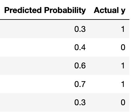
Suppose you fit a logistic regression classifier. The classifier’s predictions on a test set of 5 points are shown below, along with the actual labels.

Recall that for logistic regression, we must also choose a threshold \tau to convert the predicted probabilities to predicted labels. For this question, assume that 0 < \tau < 1. Precision is undefined when the classifier doesn’t make any positive predictions (since \frac{0}{0} is undefined). In each part, show your work and draw a box around your final answer. Each of your final answers should be a single number.
What is the lowest possible precision for any threshold \tau?
Answer: \boxed{\frac{3}{5}}
The lowest precision happens when \tau is less than 0.3. In this case, the classifier predicts all points are 1, which gives a precision of \frac{3}{5}.
What is the lowest possible recall for any threshold \tau?
Answer: \boxed{0}
The lowest recall happens when \tau is greater than 0.7. In this case, the classifier predicts all points are 0, which gives a recall of 0.
What is the highest possible recall if the classifier achieves a precision of 1?
Answer: \boxed{\frac{2}{3}}
If precision is 1, the threshold must be greater than 0.4. Of these thresholds, the recall is greatest when the threshold is between 0.4 and 0.6. In this case, the recall is \frac{2}{3}.