← return to study.practicaldsc.org
The problems in this worksheet are taken from past exams in similar classes. Work on them on paper, since the exams you take in this course will also be on paper.
Let \vec{x} = \begin{bmatrix} x_1 \\ x_2 \end{bmatrix}. Consider the function g(\vec{x}) = (x_1 - 3)^2 + (x_1^2 - x_2)^2.
Find \nabla g(\vec{x}), the gradient of g(\vec{x}), and use it to show that \nabla g\left( \begin{bmatrix} -1 \\ 1 \end{bmatrix} \right) = \begin{bmatrix} -8 \\ 0 \end{bmatrix}.
\nabla g(\vec{x}) = \begin{bmatrix} 2x_1 -6 + 4x_1(x_1^2 - x_2) \\ -2(x_1^2 - x_2) \end{bmatrix}
We can find \nabla g(\vec{x}) by finding the partial derivatives of g(\vec{x}):
\frac{\partial g}{\partial x_1} = 2(x_1 - 3) + 2(x_1^2 - x_2)(2 x_1) \frac{\partial g}{\partial x_2} = 2(x_1^2 - x_2)(-1) \nabla g(\vec{x}) = \begin{bmatrix} 2(x_1 - 3) + 2(x_1^2 - x_2)(2 x_1) \\ 2(x_1^2 - x_2)(-1) \end{bmatrix} \nabla g\left(\begin{bmatrix} - 1 \\ 1 \end{bmatrix}\right) = \begin{bmatrix} 2(-1 - 3) + 2((-1)^2 - 1)(2(-1)) \\ 2((-1)^2 - 1) \end{bmatrix} = \begin{bmatrix} -8 \\ 0 \end{bmatrix}.
We’d like to find the vector \vec{x}^* that minimizes g(\vec{x}) using gradient descent. Perform one iteration of gradient descent by hand, using the initial guess \vec{x}^{(0)} = \begin{bmatrix} -1 \\ 1 \end{bmatrix} and the learning rate \alpha = \frac{1}{2}. In other words, what is \vec{x}^{(1)}?
\vec x^{(1)} = \begin{bmatrix} 3 \\ 1 \end{bmatrix}
Here’s the general form of gradient descent: \vec x^{(1)} = \vec{x}^{(0)} - \alpha \nabla g(\vec{x}^{(0)})
We can substitute \alpha = \frac{1}{2} and x^{(0)} = \begin{bmatrix} -1 \\ 1 \end{bmatrix} to get: \vec x^{(1)} = \begin{bmatrix} -1 \\ 1 \end{bmatrix} - \frac{1}{2} \nabla g(\vec x ^{(0)}) \vec x^{(1)} = \begin{bmatrix} -1 \\ 1 \end{bmatrix} - \frac{1}{2} \begin{bmatrix} -8 \\ 0 \end{bmatrix}
\vec{x}^{(1)} = \begin{bmatrix} -1 \\ 1 \end{bmatrix} - \frac{1}{2} \begin{bmatrix} -8 \\ 0 \end{bmatrix} = \begin{bmatrix} 3 \\ 1 \end{bmatrix}
Consider the function f(t) = (t - 3)^2 + (t^2 - 1)^2. Select the true statement below.
f(t) is convex and has a global minimum.
f(t) is not convex, but has a global minimum.
f(t) is convex, but doesn’t have a global minimum.
f(t) is not convex and doesn’t have a global minimum.
f(t) is not convex, but has a global minimum.
It is seen that f(t) isn’t convex, which can be verified using the second derivative test: f'(t) = 2(t - 3) + 2(t^2 - 1) 2t = 2t - 6 + 4t^3 - 4t = 4t^3 - 2t - 6 f''(t) = 12t^2 - 2
Clearly, f''(t) < 0 for many values of t (e.g. t = 0), so f(t) is not always convex.
However, f(t) does have a global minimum – its output is never less than 0. This is because it can be expressed as the sum of two squares, (t - 3)^2 and (t^2 - 1)^2, respectively, both of which are greater than or equal to 0.
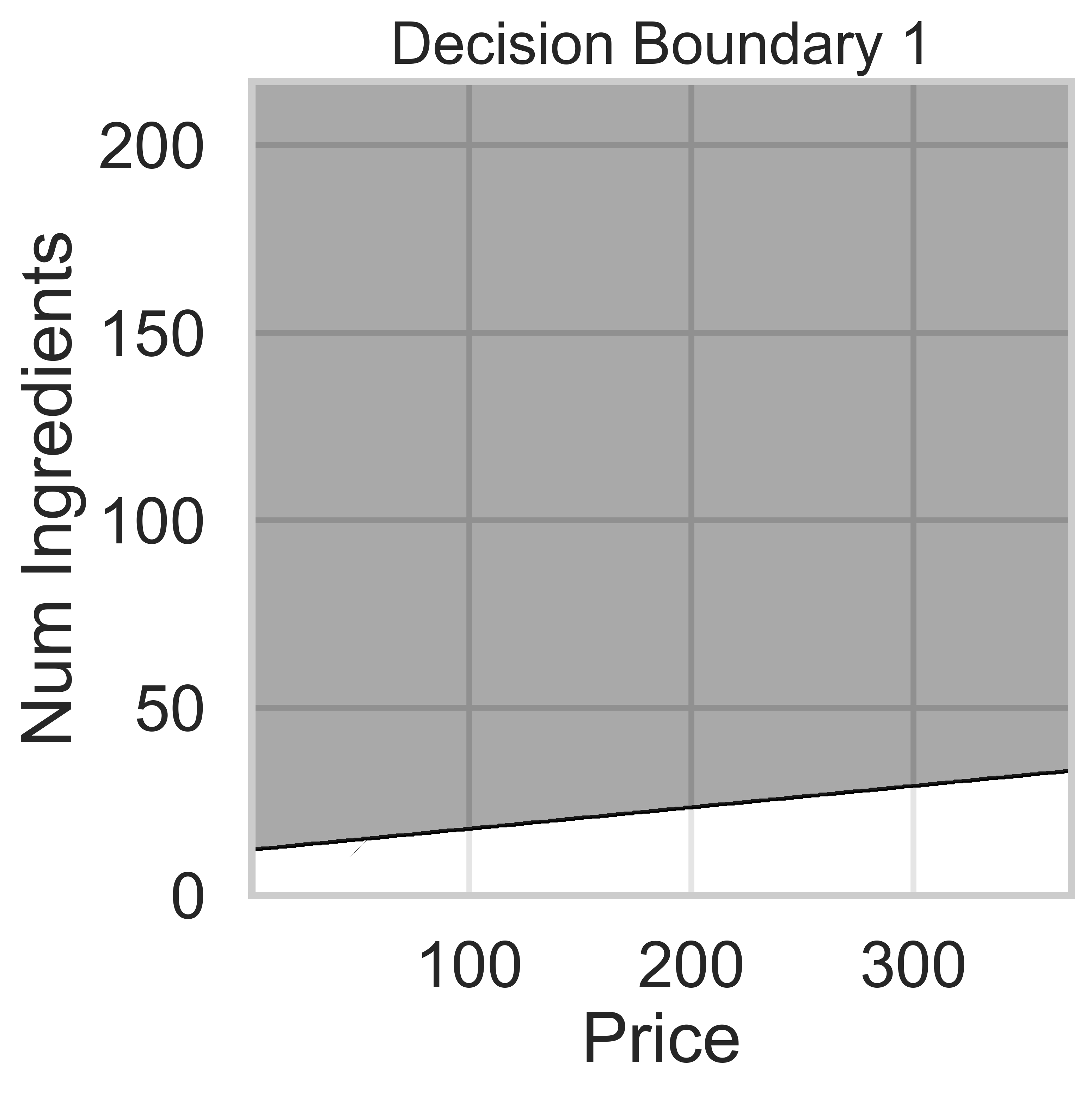
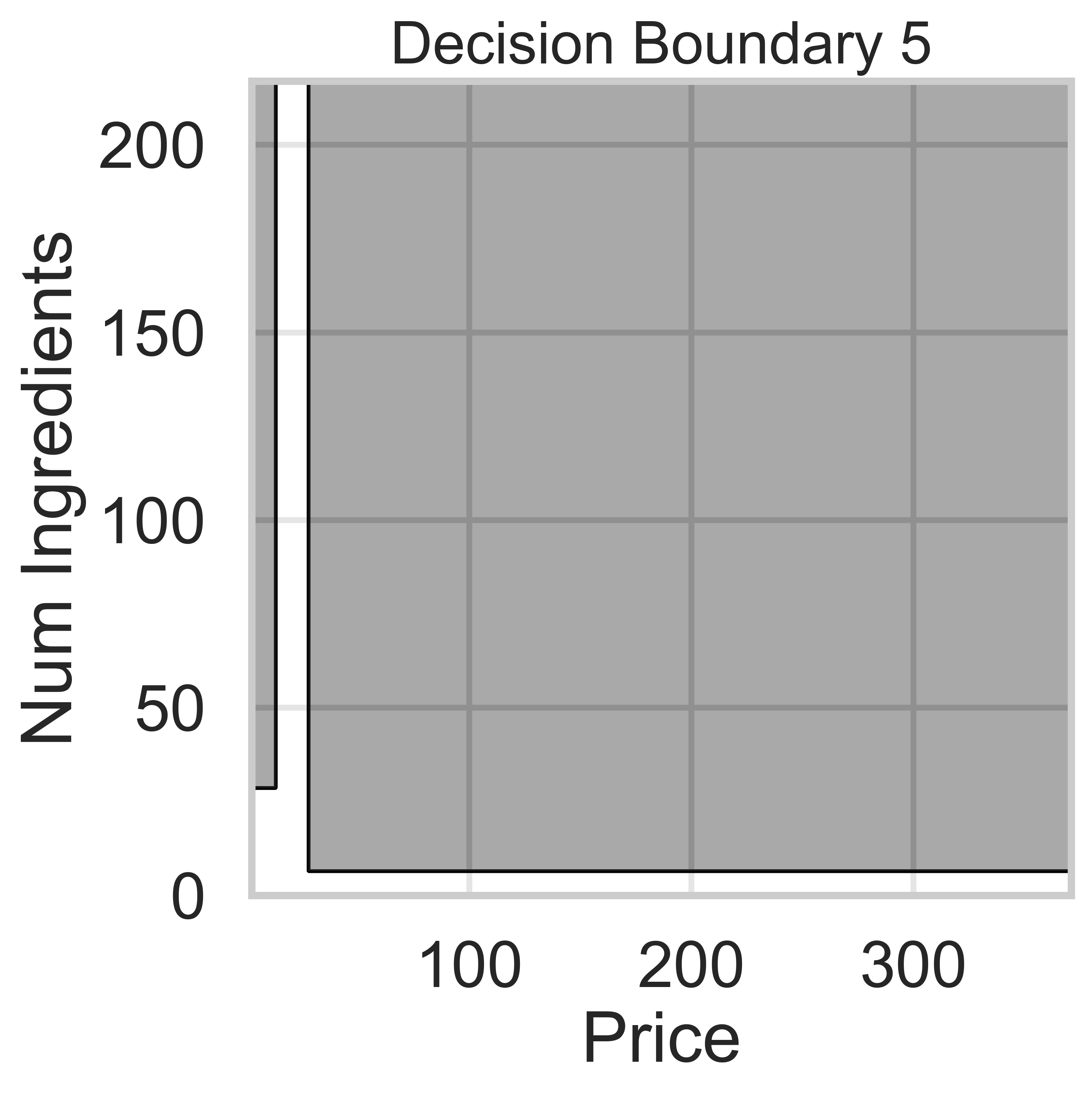
Suppose we fit five different classifiers that predict whether a product is designed for sensitive skin, given its price and number of ingredients. In the five decision boundaries below, the gray-shaded regions represent areas in which the classifier would predict that the product is designed for sensitive skin (i.e. predict class 1).
Which model does Decision Boundary 1 correspond to?
k-nearest neighbors with k = 3
k-nearest neighbors with k = 100
Decision tree with \text{max depth} = 3
Decision tree with \text{max depth} = 15
Logistic regression
Answer: Logistic regression
Logistic regression is a linear classification technique, meaning it creates a single linear decision boundary between classes. Among the five decision boundaries, only Decision Boundary 1 is linear, making it the correct answer.
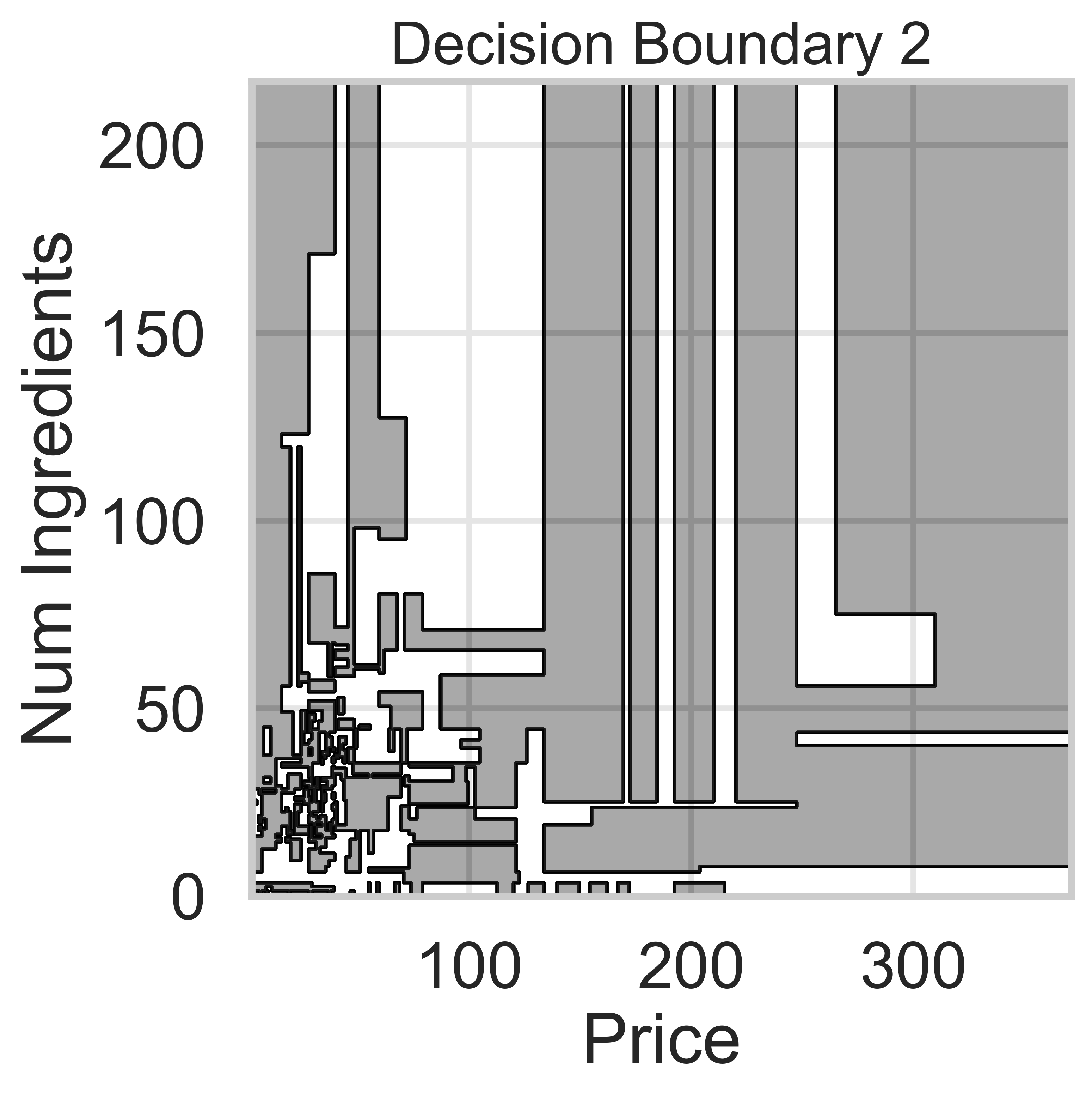
Which model does Decision Boundary 2 correspond to?
k-nearest neighbors with k = 3
k-nearest neighbors with k = 100
Decision tree with \text{max depth} = 3
Decision tree with \text{max depth} = 15
Logistic regression
Answer: Decision tree with \text{max depth} = 15
We know that Decision Boundaries 2 and 5 are decision trees, since the decision boundaries are parallel to the axes. Decision boundaries for decision trees are parallel to axes because the tree splits the feature space based on one feature at a time, creating partitions aligned with that feature’s axis (e.g., “Price ≤ 100” results in a vertical split).
Decision Boundary 2 is more complicated than Decision Boundary 5, so we can assume there are more levels.
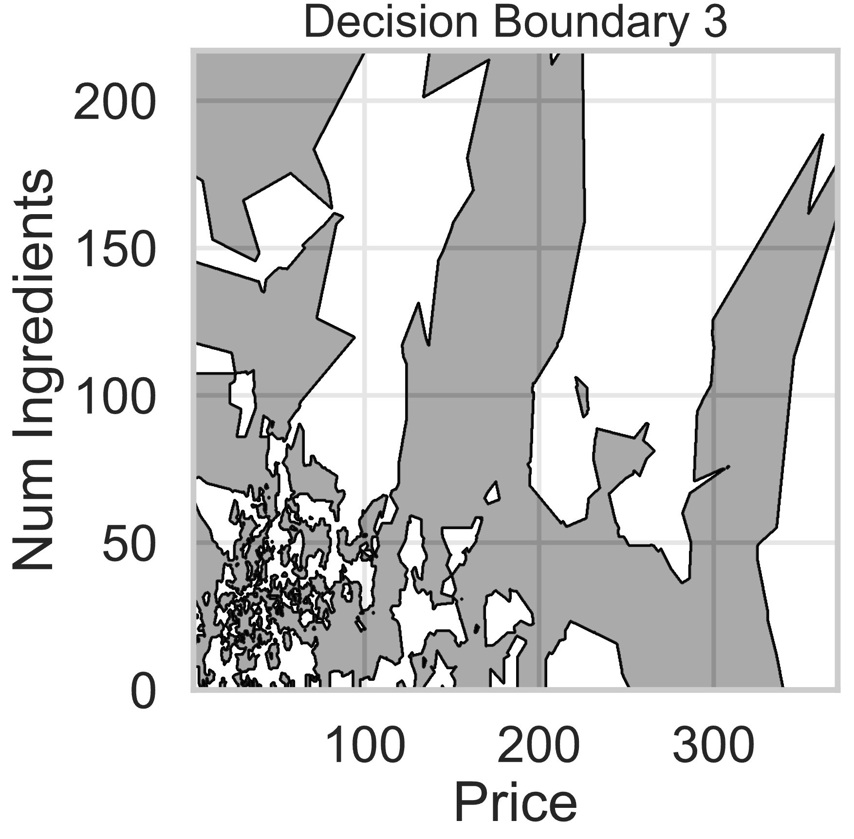
Which model does Decision Boundary 3 correspond to?
k-nearest neighbors with k = 3
k-nearest neighbors with k = 100
Decision tree with \text{max depth} = 3
Decision tree with \text{max depth} = 15
Logistic regression
Answer: k-nearest neighbors with k = 3
k-nearest neighbors decision boundaries don’t follow straight lines like logistic regression or decision trees. Thus, boundaries 3 and 4 are k-nearest neighbors.
A lower value of k means the model is more sensitive to local variations in the data. Since Decision Boundary 3 has more complex and irregular regions than Decision Boundary 4, it corresponds to k = 3, where the model closely follows the training data.
For example, if in our training data we had 3 points in the group represented by the light-shaded region at (300, 150), the decision boundary for k-nearest neighbors with k = 3 would be light-shaded at (300, 150), whereas it may be dark-shaded for k-nearest neighbors with k = 100.
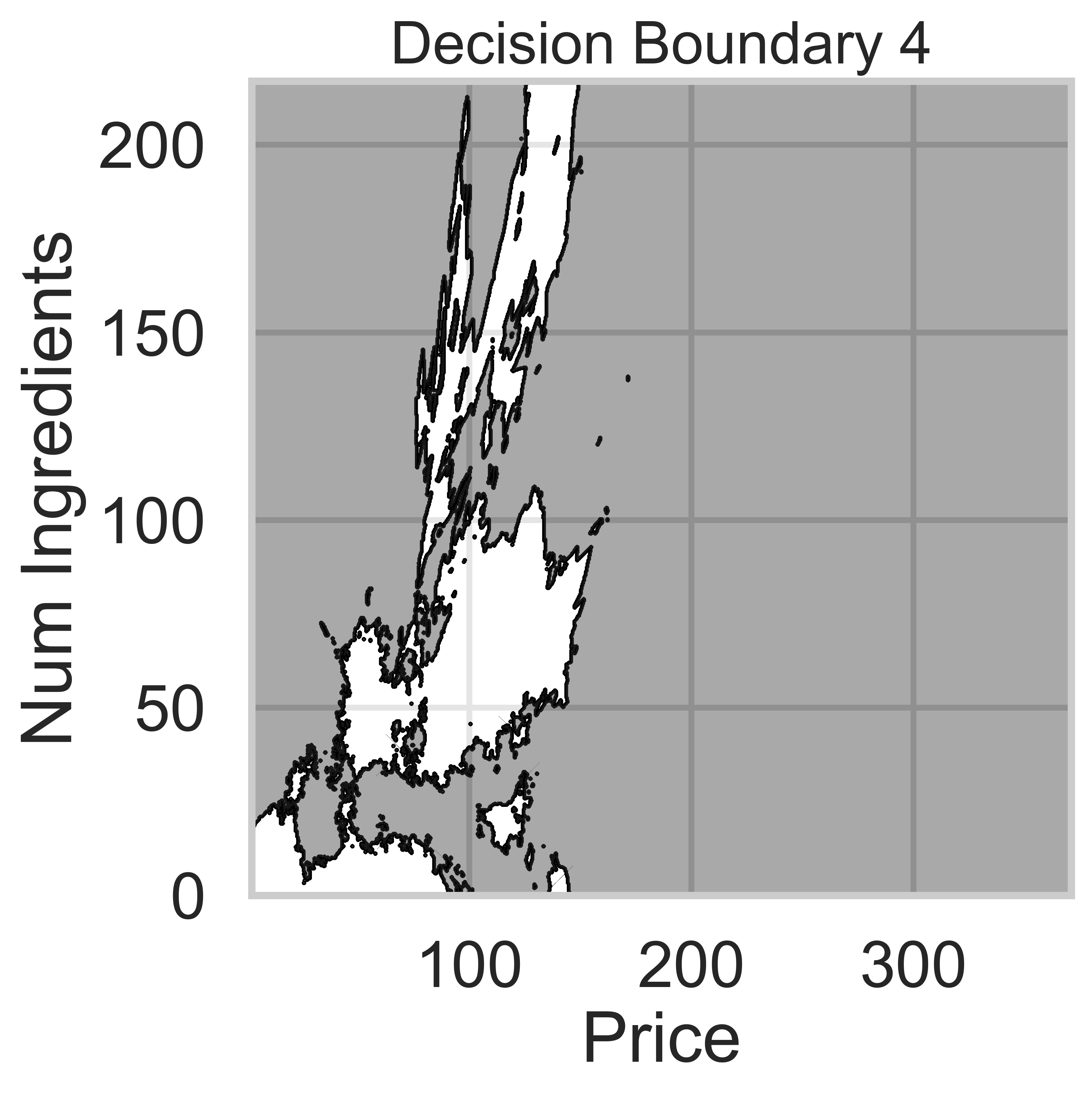
Which model does Decision Boundary 4 correspond to?
k-nearest neighbors with k = 3
k-nearest neighbors with k = 100
Decision tree with \text{max depth} = 3
Decision tree with \text{max depth} = 15
Logistic regression
Answer: k-nearest neighbors with k = 100
k-nearest neighbors decision boundaries don’t follow straight lines like logistic regression or decision trees. Thus, boundaries 3 and 4 are k-nearest neighbors.
k-nearest neighbors decision boundaries adapt to the training data, but increasing k makes the model less sensitive to local variations.
Since Decision Boundary 4 is smoother and has fewer regions than Decision Boundary 3, it corresponds to k = 100, where predictions are averaged over a larger number of neighbors, making the boundary less sensitive to individual data points.
After fitting a BillyClassifier on our training set, we
use it to make predictions on an unseen test set. Our results are
summarized in the following confusion matrix.
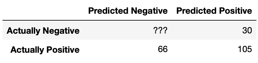
What is the recall of our classifier? Give your answer as a fraction (it does not need to be simplified).
Answer: \frac{35}{57}
There are 105 true positives and 66 false negatives. Hence, the recall is \frac{105}{105 + 66} = \frac{105}{171} = \frac{35}{57}.
The accuracy of our classifier is \frac{69}{117}. How many true negatives did our classifier have? Give your answer as an integer.
Answer: 33
Let x be the number of true negatives. The number of correctly classified data points is 105 + x, and the total number of data points is 105 + 30 + 66 + x = 201 + x. Hence, this boils down to solving for x in \frac{69}{117} = \frac{105 + x}{201 + x}.
It may be tempting to cross-multiply here, but that’s not necessary (in fact, we picked the numbers specifically so you would not have to)! Multiply \frac{69}{117} by \frac{2}{2} to yield \frac{138}{234}. Then, conveniently, setting x = 33 in \frac{105 + x}{201 + x} also yields \frac{138}{234}, so x = 33 and hence the number of true negatives our classifier has is 33.
True or False: In order for a binary classifier’s precision and recall to be equal, the number of mistakes it makes must be an even number.
True
False
Answer: True
Remember that \text{precision} = \frac{TP}{TP + FP} and \text{recall} = \frac{TP}{TP + FN}. In order for precision to be the same as recall, it must be the case that FP = FN, i.e. that our classifier makes the same number of false positives and false negatives. The only kinds of “errors" or”mistakes" a classifier can make are false positives and false negatives; thus, we must have
\text{mistakes} = FP + FN = FP + FP = 2 \cdot FP
2 times any integer must be an even integer, so the number of mistakes must be even.
Suppose we are building a classifier that listens to an audio source (say, from your phone’s microphone) and predicts whether or not it is Soulja Boy’s 2008 classic “Kiss Me thru the Phone”. Our classifier is pretty good at detecting when the input stream is “Kiss Me thru the Phone”, but it often incorrectly predicts that similar sounding songs are also “Kiss Me thru the Phone”.
Complete the sentence: Our classifier has…
low precision and low recall.
low precision and high recall.
high precision and low recall.
high precision and high recall.
Answer: Option B: low precision and high recall.
Our classifier is good at identifying when the input stream is “Kiss Me thru the Phone”, i.e. it is good at identifying true positives amongst all positives. This means it has high recall.
Since our classifier makes many false positive predictions – in other words, it often incorrectly predicts “Kiss Me thru the Phone” when that’s not what the input stream is – it has many false positives, so its precision is low.
Thus, our classifier has low precision and high recall.
We decide to build a classifier that takes in a state’s demographic information and predicts whether, in a given year:
The state’s mean math score was greater than its mean verbal score (1), or
the state’s mean math score was less than or equal to its mean verbal score (0).
The simplest possible classifier we could build is one that predicts the same label (1 or 0) every time, independent of all other features.
Consider the following statement:
If a > b, then the constant classifier that
maximizes training accuracy predicts 1 every time; otherwise, it
predicts 0 every time.
For which combination of a and b is the
above statement not guaranteed to be true?
Note: Treat sat as our training set.
Option 1:
a = (sat['Math'] > sat['Verbal']).mean()
b = 0.5
Option 2:
a = (sat['Math'] - sat['Verbal']).mean()
b = 0
Option 3:
a = (sat['Math'] - sat['Verbal'] > 0).mean()
b = 0.5
Option 4:
a = ((sat['Math'] / sat['Verbal']) > 1).mean() - 0.5
b = 0
Option 1
Option 2
Option 3
Option 4
Answer: Option 2
Conceptually, we’re looking for a combination of a and
b such that when a > b, it’s true that
in more than 50% of states, the "Math" value is
larger than the "Verbal" value. Let’s look at all
four options through this lens:
sat['Math'] > sat['Verbal'] is a Series of
Boolean values, containing True for all states where the
"Math" value is larger than the "Verbal" value
and False for all other states. The mean of this series,
then, is the proportion of states satisfying this criteria, and since
b is 0.5, a > b is
True only when the bolded condition above is
True.sat['Math'] / sat['Verbal'] is a Series that
contains values greater than 1 whenever a state’s "Math"
value is larger than its "Verbal" value and less than or
equal to 1 in all other cases. As in the other options that work,
(sat['Math'] / sat['Verbal']) > 1 is a Boolean Series
with True for all states with a larger "Math"
value than "Verbal" values; a > b compares
the proportion of True values in this Series to 0.5. (Here,
p - 0.5 > 0 is the same as p > 0.5.)Then, by process of elimination, Option 2 must be the correct option
– that is, it must be the only option that doesn’t
work. But why? sat['Math'] - sat['Verbal'] is a Series
containing the difference between each state’s "Math" and
"Verbal" values, and .mean() computes the mean
of these differences. The issue is that here, we don’t care about
how different each state’s "Math" and
"Verbal" values are; rather, we just care about the
proportion of states with a bigger "Math" value than
"Verbal" value. It could be the case that 90% of states
have a larger "Math" value than "Verbal"
value, but one state has such a big "Verbal" value that it
makes the mean difference between "Math" and
"Verbal" scores negative. (A property you’ll learn about in
future probability courses is that this is equal to the difference in
the mean "Math" value for all states and the mean
"Verbal" value for all states – this is called the
“linearity of expectation” – but you don’t need to know that to answer
this question.)
Suppose we train a classifier, named Classifier 1, and it achieves an accuracy of \frac{5}{9} on our training set.
Typically, root mean squared error (RMSE) is used as a performance metric for regression models, but mathematically, nothing is stopping us from using it as a performance metric for classification models as well.
What is the RMSE of Classifier 1 on our training set? Give your answer as a simplified fraction.
Answer: \frac{2}{3}
An accuracy of \frac{5}{9} means that the model is such that out of 9 values, 5 are labeled correctly. By extension, this means that 4 out of 9 are not labeled correctly as 0 or 1.
Remember, RMSE is defined as
\text{RMSE} = \sqrt{\frac{1}{n} \sum_{i = 1}^n (y_i - H(x_i))^2}
where y_i represents the ith actual value and H(x_i) represents the ith prediction. Here, y_i is either 0 or 1 and $H(x_i) is also either 0 or 1. We’re told that \frac{5}{9} of the time, y_i and H(x_i) are the same; in those cases, (y_i - H(x_i))^2 = 0^2 = 0. We’re also told that \frac{4}{9} of the time, y_i and H(x_i) are different; in those cases, (y_i - H(x_i))^2 = 1. So,
\text{RMSE} = \sqrt{\frac{5}{9} \cdot 0 + \frac{4}{9} \cdot 1} = \sqrt{\frac{4}{9}} = \frac{2}{3}
While Classifier 1’s accuracy on our training set is \frac{5}{9}, its accuracy on our test set is \frac{1}{4}. Which of the following scenarios is most likely?
Classifier 1 overfit to our training set; we need to increase its complexity.
Classifier 1 overfit to our training set; we need to decrease its complexity.
Classifier 1 underfit to our training set; we need to increase its complexity.
Classifier 1 underfit to our training set; we need to decrease its complexity.
Answer: Option 2
Since the accuracy of Classifier 1 is much higher on the dataset used to train it than the dataset it was tested on, it’s likely Classifer 1 overfit to the training set because it was too complex. To fix the issue, we need to decrease its complexity, so that it focuses on learning the general structure of the data in the training set and not too much on the random noise in the training set.
For the remainder of this question, suppose we train another classifier, named Classifier 2, again on our training set. Its performance on the training set is described in the confusion matrix below. Note that the columns of the confusion matrix have been separately normalized so that each has a sum of 1.
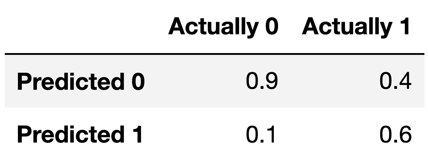
Suppose conf is the DataFrame above. Which of the
following evaluates to a Series of length 2 whose only unique value is
the number 1?
conf.sum(axis=0)
conf.sum(axis=1)
Answer: Option 1
Note that the columns of conf sum to 1 – 0.9 + 0.1 = 1, and 0.4 + 0.6 = 1. To create a Series with just
the value 1, then, we need to sum the columns of conf,
which we can do using conf.sum(axis=0).
conf.sum(axis=1) would sum the rows of
conf.
Fill in the blank: the ___ of Classifier 2 is guaranteed to be 0.6.
precision
recall
Answer: recall
The number 0.6 appears in the bottom-right corner of
conf. Since conf is column-normalized, the
value 0.6 represents the proportion of values in the second column that
were predicted to be 1. The second column contains values that were
actually 1, so 0.6 is really the proportion of values that were
actually 1 that were predicted to be 1, that is, \frac{\text{actually 1 and predicted
1}}{\text{actually 1}}. This is the definition of recall!
If you’d like to think in terms of true positives, etc., then remember that: - True Positives (TP) are values that were actually 1 and were predicted to be 1. - True Negatives (TN) are values that were actually 0 and were predicted to be 0. - False Positives (FP) are values that were actually 0 and were predicted to be 1. - False Negatives (FN) are values that were actually 1 and were predicted to be 0.
Recall is \frac{\text{TP}}{\text{TP} + \text{FN}}.
For your convenience, we show the column-normalized confusion matrix from the previous page below. You will need to use the specific numbers in this matrix when answering the following subpart.
Suppose a fraction \alpha of the labels in the training set are actually 1 and the remaining 1 - \alpha are actually 0. The accuracy of Classifier 2 is 0.65. What is the value of \alpha?
Hint: If you’re unsure on how to proceed, here are some guiding questions:
Suppose the number of y-values that are actually 1 is A and that the number of y-values that are actually 0 is B. In terms of A and B, what is the accuracy of Classifier 2? Remember, you’ll need to refer to the numbers in the confusion matrix above.
What is the relationship between A, B, and \alpha? How does it simplify your calculation for the accuracy in the previous step?
Answer: \frac{5}{6}
Here is one way to solve this problem:
accuracy = \frac{TP + TN}{TP + TN + FP + FN}
Given the values from the confusion matrix:
accuracy = \frac{0.6 \cdot \alpha + 0.9
\cdot (1 - \alpha)}{\alpha + (1 - \alpha)}
accuracy = \frac{0.6 \cdot \alpha + 0.9 - 0.9
\cdot \alpha}{1}
accuracy = 0.9 - 0.3 \cdot \alpha
Therefore:
0.65 = 0.9 - 0.3 \cdot \alpha
0.3 \cdot \alpha = 0.9 - 0.65
0.3 \cdot \alpha = 0.25
\alpha = \frac{0.25}{0.3}
\alpha = \frac{5}{6}
Consider the dataset of four values, y_1 = -2, y_2 = -1, y_3 = 2, y_4 = 4. Suppose we’d like to use gradient descent to find the constant prediction, h^*, that minimizes mean squared error on this dataset.
Write down the expression of mean square error and its derivative given this dataset.
R_\text{sq}(h) = \dfrac{1}{4}\sum_{i=1}^{4}(y_i-h)^2
Recall the equation for R_\text{sq}(h) = \frac{1}{n}\sum_{i=1}^{n}(y_i-h)^2, so we simply need to replace n with 4 because there are 4 elements in our dataset.
\frac{dR_\text{sq}(h)}{dh} = \frac{1}{2}\sum_{i=1}^{4}(h-y_i)
Since we have the equation for R_\text{sq}(h) we can calculate the derivative:
\begin{align*} \frac{dR_\text{sq}(h)}{dh} &= \frac{dR_\text{sq}(h)}{dh}(\frac{1}{4}\sum_{i=1}^{4}(y_i-h)^2) \\ &= \frac{1}{4}\sum_{i=1}^{4}\frac{dR_\text{sq}(h)}{dh}((y_i-h)^2) \\ \end{align*} We can use the chain rule to find the derivative of (y_i-h)^2. Recall the chain rule is: \frac{df(x)}{dx}[(f(x))^n] = n(f(x))^{n-1} \cdot f'(x).
\begin{align*} &= \frac{1}{4}\sum_{i=1}^{4}2(y_i-h) \cdot -1 \\ &= \frac{1}{4}\sum_{i=1}^{4} 2(h - y_i) \\ &= \frac{1}{2}\sum_{i=1}^{4} (h-y_i) \end{align*}
Suppose you choose an initial guess of h^{(0)} and a learning rate of \alpha = \frac{1}{4}. After two gradient descent steps, h^{(2)} = \frac{1}{4}. What is the value of h^{(0)}?
h^{(0)} = -\frac{5}{4}
The gradient descent equation is given by: \begin{aligned} h^{(t)} &= h^{(t-1)} - \alpha \frac{dR_{sq}(h^{(t-1)})}{dh} \end{aligned}
Recall the learning rate is equal to \alpha. We can plug in \alpha = \frac{1}{4}, h^{(2)} = \frac{1}{4}, and i=2, in that case we obtain: \begin{aligned} \frac{1}{4} &= h^{(1)} - \alpha \frac{dR_{sq}(h^{(1)})}{dh}\\ &= h^{(1)} - \alpha \frac{1}{2}\sum_{i=1}^{4}(h^{(1)}-y^{(i)})\\ &= h^{(1)} - \frac{1}{4} \cdot \frac{1}{2}(h^{(1)} + 2 + h^{(1)} + 1 + h^{(1)} - 2 + h^{(1)} - 4)\\ &= h^{(1)} - \frac{1}{8}(4h^{(1)} - 3)\\ \end{aligned}
Solving this equation, we obtain that h^{(1)} = -\frac{1}{4}. We can then repeat this step once more to obtain h^{(0)}: \begin{aligned} -\frac{1}{4} &= h^{(0)} - \alpha \frac{dR_{sq}(h^{(0)})}{dh}\\ &= h^{(0)} - \frac{1}{4} \cdot \frac{1}{2}(h^{(0)} + 2 + h^{(0)} + 1 + h^{(0)} - 2 + h^{(0)} - 4)\\ &= h^{(0)} - \frac{1}{8}(4h^{(0)} - 3)\\ \end{aligned}
Solving this equation, we obtain that h^{(0)} = -\frac{5}{4}.
Suppose we’d like to use gradient descent to minimize the function f(x) = x^3 + x^2. Suppose we choose a learning rate of \alpha = \frac{1}{4}.
Suppose x^{(t)} is our guess of the minimizing input x^{*} at timestep t, i.e. x^{(t)} is the result of performing t iterations of gradient descent, given some initial guess. Write an expression for x^{(t+1)}. Your answer should be an expression involving x^{(t)} and some constants.
In general, the update rule for gradient descent is: x^{(t+1)} = x^{(t)} - \alpha \nabla f(x^{(t)}) = x^{(t)} - \alpha \frac{df}{dx}(x^{(t)}), where \alpha is the learning rate or step size. We know that the derivative of f is as follows: \frac{df}{dx} = f'(x) = 3x^2 + 2x, thus the update rule can be written down as: x^{(t+1)} = x^{(t)} - \alpha(3x^{(t)^2} + 2x^{(t)}) = -\frac{3}{4}x^{(t)^2} + \frac{1}{2}x^{(t)}.
Suppose x^{(0)} = -1.
What is the value of x^{(1)}?
Will gradient descent eventually converge, given the initial guess x^{(0)} = -1 and step size \alpha = \frac{1}{4}?
We have f'(x^{(0)}) = f'(-1) = 3(-1)^2 + 2(-1) = 1 > 0, so we go left, and x^{(1)} = x^{(0)} - \alpha f'(x^{(0)}) = -1 - \frac{1}{4} = -\frac{5}{4}. Intuitively, the gradient descent cannot converge in this case because \text{lim}_{x \rightarrow -\infty} f(x) = -\infty,
We need to find all local minimums and local maximums. First, we solve the equation f'(x) = 0 to find all critical points.
We have: f'(x) = 0 \Leftrightarrow 3x^2 + 2x = 0 \Leftrightarrow x = -\frac{2}{3} \ \ \text{and} \ \ x = 0.
Now, we consider the second-order derivative: f''(x) = \frac{d^2f}{dx^2} = 6x + 2.
We have f''(x) = 0 only when x = -1/3. Thus, for x < -1/3, f''(x) is negative or the slope f'(x) decreases; and for x > -1/3, f''(x) is positive or the slope f'(x) increases. Keep in mind that -1 < -2/3 < -1/3 < 0 < 1.
Therefore, f has a local maximum at x = -2/3 and a local minimum at x = 0. If the gradient descent starts at x^{(0)} = -1 and it always goes left then it will never meet the local minimum at x = 0, and it will go left infinitely. We say the gradient descent cannot converge, or is divergent.
Suppose x^{(0)} = 1.
What is the value of x^{(1)}?
Will gradient descent eventually converge, given the initial guess x^{(0)} = 1 and step size \alpha = \frac{1}{4}?
We have f'(x^{(0)}) = f'(-1) = 3 \cdot 1^2 + 2 \cdot 1 = 5 > 0, so we go left, and x^{(1)} = x^{(0)} - \alpha f'(x^{(0)}) = 1 - \frac{1}{4} \cdot 5 = -\frac{1}{4}.
From the previous part, function f has a local minimum at x = 0, so the gradient descent can converge (given appropriate step size) at this local minimum.
Suppose we want to minimize the function
R(h) = e^{(h + 1)^2}
Without using gradient descent or calculus, what is the value h^* that minimizes R(h)?
h^* = -1
The minimum possible value of the exponent is 0, since anything squared is non-negative. The exponent is 0 when (x+1)^2 = 0, i.e. when x = -1. Since e^{(x+1)^2} gets larger as (x+1)^2 gets larger, the minimizing input h^* is -1.
Now, suppose we want to use gradient descent to minimize R(h). Assume we use an initial guess of h^{(0)} = 0. What is h^{(1)}? Give your answer in terms of a generic step size, \alpha, and other constants. (e is a constant.)
h^{(1)} = -\alpha \cdot 2e
First, we find \frac{dR}{dh}(h):
\frac{dR}{dh}(h) = 2(h+1) e^{(h+1)^2}
Then, we know that
h^{(1)} = h^{(0)} - \alpha \frac{dR}{dh}(h^{(0)}) = 0 - \alpha \frac{dR}{dh}(0)
In our case, \frac{dR}{dh}(0) = 2(0 + 1) e^{(0+1)^2} = 2e, so
h^{(1)} = -\alpha \cdot 2e
Using your answers from the previous two parts, what should we set the value of \alpha to be if we want to ensure that gradient descent finds h^* after just one iteration?
\alpha = \frac{1}{2e}
We know from the part 2 that h^{(1)} = -\alpha \cdot 2e, and we know from part 1 that h^* = -1. If gradient descent converges in one iteration, that means that h^{(1)} = h^*; solving this yields
-\alpha \cdot 2e = -1 \implies \alpha = \frac{1}{2e}
Below is a graph of R(h) with no axis labels.
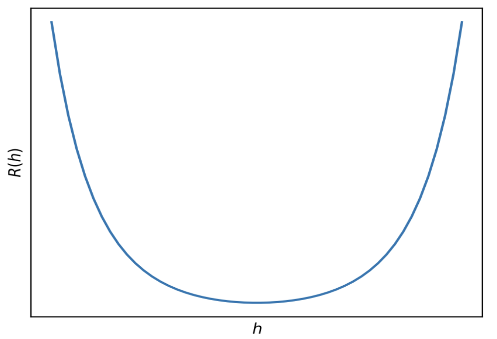
True or False: Given an appropriate choice of step size, \alpha, gradient descent is guaranteed to find the minimizer of R(h).
True.
R(h) is convex, since the graph is bowl shaped. (It can also be proved that R(h) is convex using the second derivative test.) It is also differentiable, as we saw in part 2. As a result, since it’s both convex and differentiable, gradient descent is guaranteed to be able to minimize it given an appropriate choice of step size.
Consider the function R(h) = \sqrt{(h - 3)^2 + 1} = ((h - 3)^2 + 1)^{\frac{1}{2}}, which is a convex and differentiable function with only one local minimum.
Perform by hand two iterations of the gradient descent algorithm on this function, using an initial prediction of h^{(0)} = 2 and a learning rate of \alpha = 2\sqrt{2}. Show your work and your final answers, h^{(1)} and h^{(2)}.
h^{(1)} = 4, h^{(2)} = 2
The updating rule for gradient descent in the one-dimensional case is: h^{(t+1)} = h^{(t)} - \alpha \cdot \frac{dR}{dh}(h^{(t)})
We can find \frac{dR}{dh} by taking the derivative of R(h): \frac{d}{dh}R(h) = \frac{d}{dh}(\sqrt{(h - 3)^2 + 1}) = \dfrac{h-3}{\sqrt{\left(h-3\right)^2+1}}
Now we can use \alpha = 2\sqrt{2} and h^{(0)} = 2 to begin updating:
\begin{align*}
h^{(1)} &= h^{(0)} - \alpha \cdot \frac{dR}{dh}(h^{(0)}) \\
h^{(1)} &= 2 - 2\sqrt{2} \cdot
\left(\dfrac{2-3}{\sqrt{\left(2-3\right)^2+1}}\right) \\
h^{(1)} &= 2 - 2\sqrt{2} \cdot (\dfrac{-1}{\sqrt{2}}) \\
h^{(1)} &= 4
\end{align*}
\begin{align*}
h^{(2)} &= h^{(1)} - \alpha \cdot \frac{dR}{dh}(h^{(1)}) \\
h^{(2)} &= 4 - 2\sqrt{2} \cdot
\left(\dfrac{4-3}{\sqrt{\left(4-3\right)^2+1}}\right) \\
h^{(2)} &= 4 - 2\sqrt{2} \cdot (\dfrac{1}{\sqrt{2}}) \\
h^{(2)} &= 2
\end{align*}
With more iterations, will we eventually converge to the minimizer? Explain.
No, this algorithm will not converge to the minimizer because if we do more iterations, we’ll keep oscillating back and forth between predictions of 2 and 4. We showed the first two iterations of the algorithm in part 1, but the next two would be exactly the same, and the two after that, and so on. This happens because the learning rate is too big, resulting in steps that are too big, and we keep jumping over the true minimizer at h^* = 3.
For a given classifier, suppose the first 10 predictions of our classifier and 10 true observations are as follows: \begin{array}{|c|c|c|c|c|c|c|c|c|c|c|} \hline \textbf{Predictions} & 1 & 1 & 1 & 1 & 1 & 0 & 1 & 1 & 1 & 1 \\ \hline \textbf{True Label} & 0 & 1 & 1 & 1 & 0 & 0 & 0 & 1 & 1 & 1 \\ \hline \end{array}
What is the accuracy of our classifier on these 10 predictions?
What is the precision on these 10 predictions?
What is the recall on these 10 predictions?
Answer:
Let’s first identify all elements of the confusion matrix by comparing predictions with true labels:
| Metric | Count | Explanation |
|---|---|---|
| True Positives (TP) | 6 | Prediction=1 and True Label=1 |
| False Positives (FP) | 3 | Prediction=1 and True Label=0 |
| True Negatives (TN) | 1 | Prediction=0 and True Label=0 |
| False Negatives (FN) | 0 | Prediction=0 and True Label=1 |
| Total | 10 | Total number of predictions |
Accuracy: The proportion of correct predictions (TP + TN) among the total number of predictions. \text{Accuracy} = \frac{TP + TN}{TP + TN + FP + FN} = \frac{6 + 1}{10} = \frac{7}{10} = 0.7
Precision: The proportion of true positives among all positive predictions. \text{Precision} = \frac{TP}{TP + FP} = \frac{6}{6 + 3} = \frac{6}{9} = \frac{2}{3} \approx 0.67
Recall: The proportion of true positives among all actual positives. \text{Recall} = \frac{TP}{TP + FN} = \frac{6}{6 + 0} = \frac{6}{6} = 1
Consider three classifiers with the following confusion matrices:
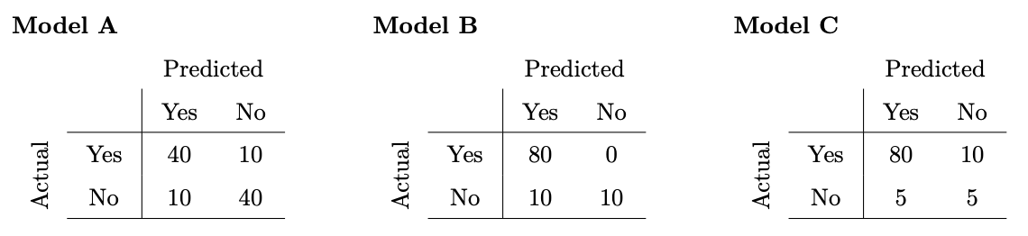
Which model has the highest accuracy?
Model A
Model B
Model C
Answer: Model B
Accuracy is defined as \frac{\text{number\;of\;correct\;predictions}}{\text{number\;of\;total\;predictions}}, so we sum the (Yes, Yes) and (No, No) cells to get the number of correct predictions and divide that by the sum of all cells as the number of total predictions. We see that Model B has the highest accuracy of 0.9 with that formula. (Note that for simplicity, the confusion matrices are such that the sum of all values is 100 in all three cases.)
Which model has the highest precision?
Model A
Model B
Model C
Answer: Model C
Precision is defined as \frac{\text{number of correctly predicted yes values}}{\text{total number of yes predictions}}, so the number of correctly predicted yes values is the (Yes, Yes) cell, while the total number of yes predictions is the sum of the Yes column. We see that Model C has the highest precision, \frac{80}{85}, with that formula.
Which model has the highest recall?
Model A
Model B
Model C
Answer: Model B
Recall is defined as \frac{\text{number of correctly predicted yes values}}{\text{total number of values actually yes}}, so the number of correctly predicted yes values is the (Yes, Yes) cell, while the total number of values that are actually yes is the sum of the Yes row. We see that Model B has the highest recall, 1, with that formula.
Suppose Yutong builds a classifier that predicts whether or not a hotel provides free parking. The confusion matrix for her classifier, when evaluated on our training set, is given below.
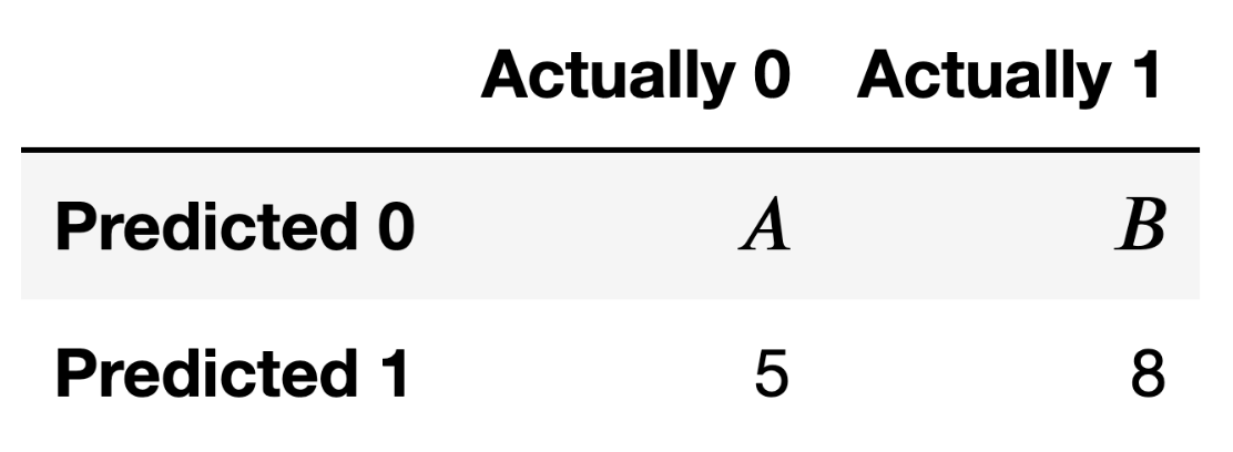
What is the precision of Yutong’s classifier? Give your answer as a simplified fraction.
Answer: \frac{8}{13}
Precision is the proportion of predicted positives that actually were positives. So, given this confusion matrix, that value is \frac{8}{8 + 5}, or \frac{8}{13}.
Fill in the blanks: In order for Yutong’s classifier’s recall to be
equal to its precision, __(i)__ must be equal to
__(ii)__.
A
B
2
3
4
5
6
8
13
14
20
40
50
80
Answer:
We already know that the precision is \frac{8}{13}. Recall is the proportion of true positives that were indeed classified positives, which in this matrix is \frac{8}{B + 8}. So, in order for precision to equal recall, B must be 5.
Now, suppose both A and B are unknown. Fill in the blanks: In order
for Yutong’s classifier’s recall to be equal to its accuracy,
__(i)__ must be equal to __(ii)__.
A + B
A - B
B - A
A \cdot B
\frac{A}{B}
\frac{B}{A}
2
3
4
5
6
8
13
14
20
40
50
80
Hint: To verify your answer, pick an arbitrary value of A, like A = 10, and solve for the B that sets the model’s recall equal to its accuracy. Do the specific A and B you find satisfy your answer above?
Answer:
We can solve this problem by simply stating recall and accuracy in terms of the values in the confusion matrix. As we already found, recall is \frac{8}{B+8}. Accuracy is the sum of correct predictions over total number of predictions, or \frac{A + 8}{A + B + 13}. Then, we simply set these equal to each other, and solve.
\frac{8}{B+8} = \frac{A + 8}{A + B + 13} 8(A + B + 13) = (A + 8)(B + 8) 8A + 8B + 104 = AB + 8A + 8B + 64 104 = AB + 64 AB = 40