← return to study.practicaldsc.org
The problems in this worksheet are taken from past exams in similar classes. Work on them on paper, since the exams you take in this course will also be on paper.
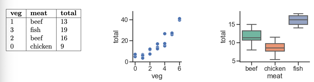
Every week, Lauren goes to her local grocery store and buys a varying amount of vegetable but always buys exactly one pound of meat (either beef, fish, or chicken). We use a linear regression model to predict her total grocery bill. We’ve collected a dataset containing the pounds of vegetables bought, the type of meat bought, and the total bill. Below we display the first few rows of the dataset and two plots generated using the entire training set.
Suppose we fit the following linear regression models to predict
'total' using the squared loss function. Based on the data
and visualizations shown above, for each of the following models H(x_i), determine whether each fitted
model coefficient w^* is
positive (+), negative (-), or exactly 0. The notation \text{meat=beef} refers to the one-hot
encoded 'meat' column with value 1 if the original value in the
'meat' column was 'beef' and 0 otherwise. Likewise, \text{meat=chicken} and \text{meat=fish} are the one-hot encoded
'meat' columns for 'chicken' and
'fish', respectively.
For example, in part (iv), you’ll need to provide three answers: one for w_0^* (either positive, negative, or 0), one for w_1^* (either positive, negative, or 0), and one for w_2^* (either positive, negative, or 0).
Model i. H(x_i) =
w_0
Answer: w_0^* must be positive
If H(x_i) = w_0, then w_0^* will be the mean 'total'
value in our dataset, and since all of our observed 'total'
values are positive, their mean – and hence, w_0^* – must also be positive.
Model ii. H(x_i) = w_0 + w_1 \cdot
\text{veg}_i
Answer: w_0^* must be positive; w_1^* must be positive
Of the three graphs provided, the middle one shows the relationship
between 'total' and 'veg'. We see that if we
were to draw a line of best fit, the y-intercept (w_0^*) would be positive, and so would the
slope (w_1^*).
Model iii. H(x_i) = w_0 + w_1 \cdot
\text{(meat=chicken)}_i
Answer:
w_0^* must be positive; w_1^* must be negative
Here’s the key to solving this part (and the following few): the
input x has a 'meat' of
'chicken', H(x_i) = w_0 +
w_1. If the input x has a
'meat' of something other than 'chicken', then
H(x_i) = w_0. So:
'total' prediction that makes sense for non-chicken inputs,
and'total' prediction for chickens.For all three 'meat' categories, the average observed
'total' value is positive, so it would make sense that for
non-chickens, the constant prediction w_0^* is positive. Based on the third graph,
it seems that 'chicken's tend to have a lower
'total' value on average than the other two categories, so
if the input x is a
'chicken' (that is, if \text{meat=chicken} = 1), then the constant
'total' prediction should be less than the constant
'total' prediction for other 'meat's. Since we
want w_0^* + w_1^* to be less than w_0^*, w_1^*
must then be negative.
Model iv. H(\vec x_i) = w_0 + w_1
\cdot \text{(meat=beef)}_i + w_2 \cdot
\text{(meat=chicken)}_i
Answer:
w_0^* must be positive; w_1^* must be negative; w_2^* must be negative
H(\vec x_i) makes one of three predictions:
'meat'
value of 'chicken', then it predicts w_0 + w_2.'meat'
value of 'beef', then it predicts w_0 + w_1.'meat'
value of 'fish', then it predicts w_0.Think of w_1^* and w_2^* – the optimal w_1 and w_2
– as being adjustments to the mean 'total' amount for
'fish'. Per the third graph, 'fish' have the
highest mean 'total' amount of the three
'meat' types, so w_0^*
should be positive while w_1^* and
w_2^* should be negative.
Model v. H(\vec x_i) = w_0 + w_1
\cdot \text{(meat=beef)}_i + w_2 \cdot \text{(meat=chicken)}_i + w_3
\cdot \text{(meat=fish)}_i
Answer:
Not enough information for any of the four coefficients!
Like in the previous part, H(\vec x_i) makes one of three predictions:
'meat'
value of 'chicken', then it predicts w_0 + w_2.'meat'
value of 'beef', then it predicts w_0 + w_1.'meat'
value of 'fish', then it predicts w_0 + w_3.Since the mean minimizes mean squared error for the constant model,
we’d expect w_0^* + w_2^* to be the
mean 'total' for 'chicken', w_0^* + w_1^* to be the mean
'total' for 'beef', and w_0^* + w_3^* to be the mean total for
'fish'. The issue is that there are infinitely many
combinations of w_0^*, w_1^*, w_2^*,
w_3^* that allow this to happen!
Pretend, for example, that:
'total' for 'chicken is 8.'total' for 'beef' is 12.'total' for 'fish' is 15.Then, w_0^* = -10, w_1^* = 22, w_2^* = 18, w_3^* = 25 and w_0^* = 20, w_1^* = -8, w_2^* = -12, w_3^* = -5 work, but the signs of the coefficients are inconsistent. As such, it’s impossible to tell!
Suppose we fit the model H(\vec x_i) = w_0 + w_1 \cdot \text{veg}_i + w_2 \cdot (\text{meat=beef})_i + w_3 \cdot (\text{meat=fish})_i. After fitting, we find that \vec{w^*}=[-3, 5, 8, 12].
What is the prediction of this model on the first point in our dataset?
-3
2
5
10
13
22
25
Answer: 10
Plugging in our weights \vec{w}^* to the model H(\vec x_i) and filling in data from the row
| veg | meat | total |
|---|---|---|
| 1 | beef | 13 |
gives us -3 + 5(1) + 8(1) + 12(0) = 10.
Following the same model H(\vec x_i) and weights from the previous problem, what is the loss of this model on the second point in our dataset, using squared loss?
0
1
5
6
8
24
25
169
Answer: 25
The squared loss for a single point is (\text{actual} - \text{predicted})^2. Here,
our actual 'total' value is 19, and our predicted value
'total' value is -3 + 5(3) + 8(0)
+ 12(1) = -3 + 15 + 12 = 24, so the squared loss is (19 - 24)^2 = (-5)^2 = 25.
Suppose we want to fit a multiple linear regression model (using squared loss) that predicts the number of ingredients in a product given its price and various other information.
From the Data Overview page, we know that there are 6 different types of products. Assume in this question that there are 20 different product brands. Consider the models defined in the table below.
| Model Name | Intercept | Price | Type | Brand |
|---|---|---|---|---|
| Model A | Yes | Yes | No | One hot encoded |
without drop="first" |
||||
| Model B | Yes | Yes | No | No |
| Model C | Yes | Yes | One hot encoded | |
without drop="first" |
||||
| Model D | No | Yes | One hot encoded | One hot encoded |
with drop="first" |
with drop="first" |
|||
| Model E | No | Yes | One hot encoded | One hot encoded |
with drop="first" |
without drop="first" |
For instance, Model A above includes an intercept term, price as a
feature, one hot encodes brand names, and doesn’t use
drop="first" as an argument to OneHotEncoder
in sklearn.
In parts 1 through 3, you are given a model. For each model provided, state the number of columns and the rank (i.e. number of linearly independent columns) of the design matrix, X. Some of part 1 is already done for you as an example.
Model A
Number of columns in X:
Rank of X: 21
Answer:
Number of columns in X: 22
Model A includes an intercept, the price feature, and a one-hot encoding of the 20 brands without dropping the first category. The intercept adds 1 column, the price adds 1 column, and the one-hot encoding for brands adds 20 columns. The rank is 21 because one of the brand categories can be predicted by the others (i.e., the columns are linearly dependent).
The rank is 21 because when encoding categorical variables (such as brands), dropping the first category avoids introducing perfect multicollinearity. By not dropping a category, we increase the rank by 1, but this still maintains linear dependence among the columns.
Model B
Number of columns in X:
Rank of X:
Answer:
Number of columns in X:
2
Rank of X: 2
Model B includes an intercept and the price feature, but no one-hot encoding for the brands or product types. The intercept and price are linearly independent, resulting in both the number of columns and the rank being 2.
Model C
Number of columns in X:
Rank of X:
Answer:
Number of columns in X:
8
Rank of X: 7
Model C includes an intercept, the price feature, and a one-hot encoding of the 6 product types without dropping the first category. The intercept adds 1 column, the price adds 1 column, and the one-hot encoding for the product types adds 6 columns. However, one column is linearly dependent because we didn’t drop one of the one-hot encoded columns, reducing the rank to 7.
This happens because if we have 6 product types, one of the columns can always be written as a linear combination of the other five. Thus, we lose one degree of freedom in the matrix, and the rank is 7.
Which of the following models are NOT guaranteed to have residuals that sum to 0?
Hint: Remember, the residuals of a fit model are the differences between actual and predicted y-values, among the data points in the training set.
Model A
Model B
Model C
Model D
Model E
Answer: Model D
For residuals to sum to zero in a linear regression model, the design matrix must include either an intercept term (Models A - C) or equivalent redundancy in the encoded variables to act as a substitute for the intercept (Model E). Models that lack both an intercept and equivalent redundancy, such as Model D, are not guaranteed to have residuals sum to zero.
For a linear model, the residual vector \vec{e} is chosen such that it is orthogonal to the column space of the design matrix X. If one of the columns of X is a column of all ones (as in the case with an intercept term), it ensures that the sum of the residuals is zero. This is because the error vector \vec{e} is orthogonal to the span of X, and hence X^T \vec{e} = 0. If there isn’t a column of all ones, but we can create such a column using a linear combination of the other columns in X, the residuals will still sum to zero. Model D lacks this structure, so the residuals are not guaranteed to sum to zero.
In contrast, one-hot encoding without dropping any category can behave like an intercept because it introduces a column for each category, allowing the model to adjust its predictions as if it had an intercept term. The sum of the indicator variables in such a setup equals 1 for every row, creating a similar effect to an intercept, which is why residuals may sum to zero in these cases.
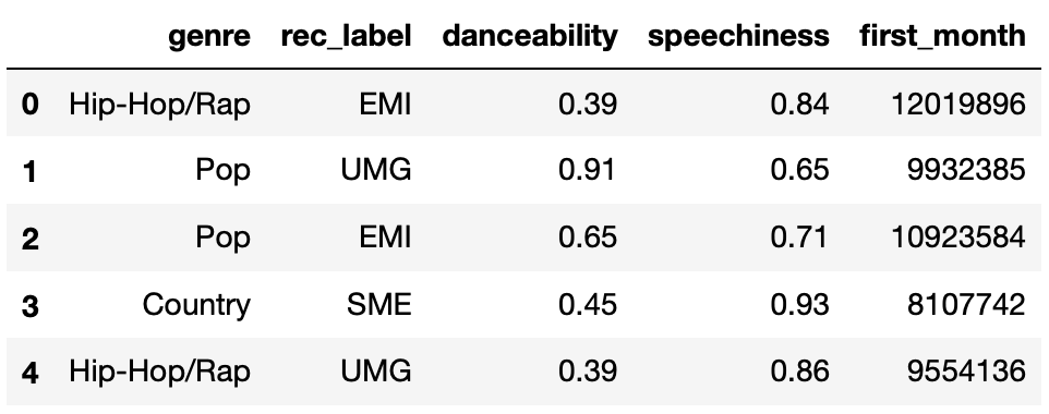
The DataFrame new_releases contains the following
information for songs that were recently released:
"genre": the genre of the song (one of the following
5 possibilities: "Hip-Hop/Rap", "Pop",
"Country", "Alternative", or
"International")
"rec_label": the record label of the artist who
released the song (one of the following 4 possibilities:
"EMI", "SME", "UMG", or
"WMG")
"danceability": how easy the song is to dance to,
according to the Spotify API (between 0 and 1)
"speechiness": what proportion of the song is made
up of spoken words, according to the Spotify API (between 0 and
1)
"first_month": the number of total streams the song
had on Spotify in the first month it was released
The first few rows of new_releases are shown below
(though new_releases has many more rows than are shown
below).
We decide to build a linear regression model that predicts
"first_month" given all other information. To start, we
conduct a train-test split, splitting new_releases into
X_train, X_test, y_train, and
y_test.
We then fit two linear models (with intercept terms) to the training data:
Model 1 (lr_one): Uses "danceability"
only.
Model 2 (lr_two): Uses "danceability"
and "speechiness" only.
Consider the following outputs.
>>> X_train.shape[0]
50

>>> np.sum((y_train - lr_two.predict(X_train)) ** 2)
500000 # five hundred thousand
What is Model 2 (lr_two)’s training RMSE (square root of
mean squared error)? Give your answer as an integer.
Answer: 100
We are given that there are n=50 data points, and that the sum of squared errors \sum_{i = 1}^n (y_i - H(x_i))^2 is 500{,}000. Then:
\begin{aligned} \text{RMSE} &= \sqrt{\frac{1}{n} \sum_{i = 1}^n (y_i - H(x_i))^2} \\ &= \sqrt{\frac{1}{50} \cdot 500{,}000} \\ &= \sqrt{10{,}000} \\ &= 100\end{aligned}
Now, suppose we fit two more linear models (with intercept terms) to the training data:
Model 3 (\texttt{lr\_drop}):
Uses "danceability" and "speechiness" as-is,
and one-hot encodes "genre" and "rec_label",
using OneHotEncoder(drop="first").
Model 4 (\texttt{lr\_no\_drop}):
Uses "danceability" and "speechiness" as-is,
and one-hot encodes "genre" and "rec_label",
using OneHotEncoder().
Note that the only difference between Model 3 and Model 4 is the fact
that Model 3 uses drop="first".
How many one-hot encoded columns are used in each model? In other words, how many binary columns are used in each model? Give both answers as integers.
Hint: Make sure to look closely at the description of
new_releases at the top of the previous page, and don’t
include the already-quantitative features.
number of one-hot encoded columns in Model 3 (lr_drop)
=
number of one-hot encoded columns in Model 4
(lr_no_drop) =
Answer: 7 and 9
There are 5 unique values of "genre" and 4 unique values
of "rec_label", so if we create a single one-hot encoded
column for each one, there would be 5 + 4 =
9 one-hot encoded columns (which there are in
lr_no_drop).
If we drop one one-hot-encoded column per category, which is what
drop="first" does, then we only have (5 - 1) + (4 - 1) = 7 one-hot encoded columns
(which there are in lr_drop).
Recall, in Model 4 (lr_no_drop) we one-hot encoded
"genre" and "rec_label", and did not use
drop="first" when instantiating our
OneHotEncoder.
Suppose we are given the following coefficients in Model 4:
The coefficient on "genre_Pop" is 2000.
The coefficient on "genre_Country" is 1000.
The coefficient on "danceability" is 10^6 = 1{,}000{,}000.
Daisy and Billy are two artists signed to the same
"rec_label" who each just released a new song with the same
"speechiness". Daisy is a "Pop" artist while
Billy is a "Country" artist.
Model 4 predicted that Daisy’s song and Billy’s song will have the
same "first_month" streams. What is the absolute
difference between Daisy’s song’s "danceability"
and Billy’s song’s "danceability"? Give your answer as a
simplified fraction.
Answer: \frac{1}{1000}
“My favorite problem on the exam!" -Suraj
Model 4 is made up of 11 features, i.e. 11 columns.
4 of the columns correspond to the different values of
"rec_label". Since Daisy and Billy have the same
"rec_label", their values in these four columns are all the
same.
One of the columns corresponds to "speechiness".
Since Daisy’s song and Billy’s song have the same
"speechiness", their values in this column are the
same.
5 of the columns correspond to the different values of
"genre". Daisy is a "Pop" artist, so she has a
1 in the "genre_Pop" column and a 0 in the other four
"genre_" columns, and similarly Billy has a 1 in the
"genre_Country" column and 0s in the others.
One of the columns corresponds to "danceability",
and Daisy and Billy have different quantitative values in this
column.
Let d_1 and d_2.
The key is in recognizing that all features in Daisy’s prediction and
Billy’s prediction are the same, other than the coefficients on
"genre_Pop", "genre_Country", and
"danceability". Let’s let d_1 be Daisy’s song’s
"danceability", and let d_2 be Billy’s song’s
"danceability". Then:
\begin{aligned} 2000 + 10^{6} \cdot d_1 = 1000 + 10^{6} \cdot d_2 \\ 1000 &= 10^{6} (d_2 - d_1) \\ \frac{1}{1000} &= d_2 - d_1\end{aligned}
Thus, the absolute difference between their songs’
"danceability"s is \frac{1}{1000}.
One piece of information that may be useful as a feature is the
proportion of SAT test takers in a state in a given year that qualify
for free lunches in school. The Series lunch_props contains
8 values, each of which are either "low",
"medium", or "high". Since we can’t use
strings as features in a model, we decide to encode these strings using
the following Pipeline:
# Note: The FunctionTransformer is only needed to change the result
# of the OneHotEncoder from a "sparse" matrix to a regular matrix
# so that it can be used with StandardScaler;
# it doesn't change anything mathematically.
pl = Pipeline([
    ("ohe", OneHotEncoder(drop="first")),
    ("ft", FunctionTransformer(lambda X: X.toarray())),
    ("ss", StandardScaler())
])
After calling pl.fit(lunch_props),
pl.transform(lunch_props) evaluates to the following
array:
array([[ 1.29099445, -0.37796447],
       [-0.77459667, -0.37796447],
       [-0.77459667, -0.37796447],
       [-0.77459667,  2.64575131],
       [ 1.29099445, -0.37796447],
       [ 1.29099445, -0.37796447],
       [-0.77459667, -0.37796447],
       [-0.77459667, -0.37796447]])
and pl.named_steps["ohe"].get_feature_names() evaluates
to the following array:
array(["x0_low", "x0_med"], dtype=object)Given the above information, we can conclude that
lunch_props has (a) value(s) equal to
"low", (b) value(s) equal to
"medium", and (c) value(s) equal to
"high". (Note: Each of (a), (b), and (c) should be
positive numbers, such that together, they add to 8.)
What are (a), (b), and (c)? Give your answers as positive integers.
Answer: 3, 1, 4
The first column of the transformed array corresponds to the
standardized one-hot-encoded low column. There are 3 values
that are positive, which means there are 3 values that were originally
1 in that column pre-standardization. This means that 3 of
the values in lunch_props were originally
"low".
The second column of the transformed array corresponds to the
standardized one-hot-encoded med column. There is only 1
value in the transformed column that is positive, which means only 1 of
the values in lunch_props was originally
"medium".
The Series lunch_props has 8 values, 3 of which were
identified as "low" in subpart 1, and 1 of which was
identified as "medium" in subpart 2. The number of values
being "high" must therefore be 8
- 3 - 1 = 4.
Suppose we have one qualitative variable that that we convert to numerical values using one- hot encoding. We’ve shown the first four rows of the resulting design matrix below:

Say we train a linear model m_1 on these data. Then, we replace all of the 1 values in column a with 3’s and all of the 1 values in column b with 2’s and train a new linear model m_2. Neither m_1 nor m_2 have an intercept term. On the training data, the average squared loss for m_1 will be ________ that of m_2.
greater than
less than
equal to
impossible to tell
Answers:
The answer is equal to.
Because we can simply adjust the weights in the opposite way that we rescale the one-hot columns, any model obtainable with the original encoding can also be obtained with the rescaled encoding. This guarantees that the training loss remains unchanged.
When one-hot encoding is used, each category is represented by a column that typically contains only 0s and 1s. Rescaling these columns means multiplying the 1s by a constant (for example, turning 1 into 2 or 3). However, if we also adjust the corresponding weights in the model by dividing by that same constant, the product of the rescaled column value and its weight remains the same. Since the model’s predictions are based on these products, the predictions will not change, and as a result, the average squared loss on the training data will also remain unchanged.
For example, let us say we have categorical variable “Color” with three levels: Red, Green, and Blue. We one-hot encode this variable into three columns. For an observation: - If the color is Red, the encoded values might be: Red = 1, Green = 0, Blue = 0.
Now, suppose we decide to multiply the column for Red by 2. The new value for a Red observation becomes 2 instead of 1. To keep the prediction the same, we can simply use half the weight for this column in the model. This inverse adjustment ensures that the final product (column value multiplied by weight) remains unchanged. Thus, the model’s prediction and the average squared loss on the training data stay the same.
To account for the intercept term, we add a column of all ones to our design matrix from part a. That is, the resulting design matrix has four columns: a with 3’s instead of 1’s, b with 2’s instead of 1’s, c, and a column of all ones. What is the rank of the new design matrix with these four columns?
1
2
3
4
Answers:
The answer is 3.
Note that the column c = intercept column −\frac{1}{3}a + \frac{1}{2}b. Hence, there is a linear dependence relationship, meaning that one of the columns is redundant and that the rank of the new design matrix is 3.
Reggie and Essie are given a dataset of real features x_i \in \mathbb{R} and observations y_i. Essie proposes the following hypothesis function: F(x_i) = \alpha_0 + \alpha_1 x_i and Reggie proposes to the following linear prediction rule: G(x_i) = \gamma_0 + \gamma_1 x_i^2
Let MMSE(F) be the minimum value of mean squared error that F achieves on a given dataset, and let MMSE(G) be the minimum value of mean squared error that G achieves on a given dataset. Give an example of a dataset (x_1, y_1), (x_2, y_2), …, (x_n, y_n) for which MMSE(F) > MMSE(G).
Example: If the datapoints follow a quadratic form y_i=x_i^2 for all i, then the G prediction rule will achieve a zero error while F>0 since the data do not follow a linear form.
Let MMSE(F) be the minimum value of mean squared error that F achieves on a given dataset, and let MMSE(G) be the minimum value of mean squared error that G achieves on a given dataset. Give an example of a dataset (x_1, y_1), (x_2, y_2), …, (x_n, y_n) for which MMSE(F) = MMSE(G).
Example 1: If the response variables are constant y_i=c for all i, then for both prediciton rules by setting \alpha_0=\gamma_0=c and \alpha_1=\gamma_1=0, both predictors will achieve MSE=0.
Example 2: when every single value of the features x_i and x^2_ i coincide in the dataset (this occurs when x = 0 or x = 1), the parameters of both prediction rules will be the same, as will the MSE.
Reggie adds a new feature x^{(2)}, to his dataset and creates two new hypothesis functions, J and K: J(\vec x_i) = w_0 + w_1 x_i^{(1)} + w_2 x_i^{(2)} K(\vec x_i) = \beta_0 + \beta_1 x_i^{(1)} + \beta_2 x_i^{(2)} + \beta_3 (2 x_i^{(1)} - x_i^{(2)}) Reggie argues that having more features is better, so MMSE(K) < MMSE(J). Is Reggie correct? Why or why not?
K(\vec x_i) can be rewritten as K(\vec x_i) = \beta_0 + (\beta_1+2\beta_3) x_i^{(1)} +(\beta_2 - \beta_3)x_i^{(2)} By setting \tilde{\beta}_1=\beta_1+2\beta_3 and \tilde{\beta_2}= \beta_2 - \beta_3 then
K(\vec x_i) = K(\beta_0,\tilde{\beta}_1,\tilde{\beta}_2) = \beta_0 + \tilde{\beta_1} x_i^{(1)} +\tilde{\beta}_2 x_i^{(2)}
Thus J and K have the same normal equations and therefore the same minimum MSE.
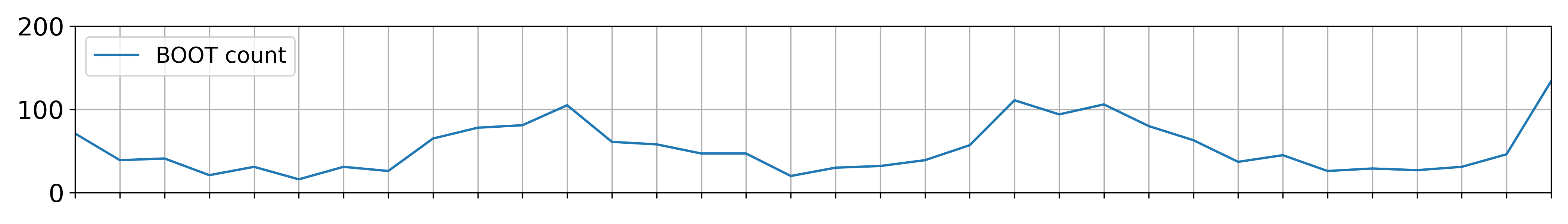
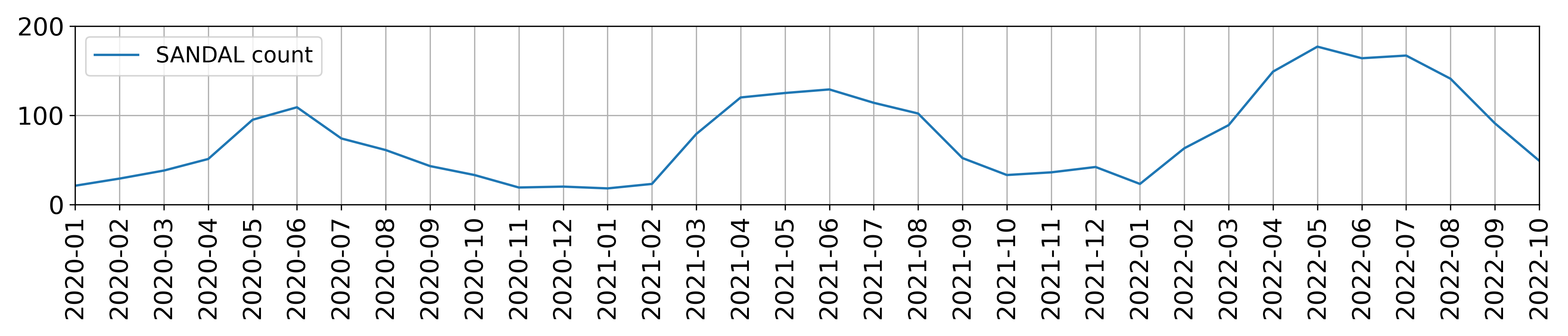
The two plots below show the total number of boots (top) and sandals
(bottom) purchased per month in the df table. Assume that
there is one data point per month.
For each of the following regression models, use the visualizations shown above to select the value that is closest to the fitted model weights. If it is not possible to determine the model weight, select “Not enough info”. For the models below:
\text{predicted boot}_i = w_0
w_0:
0
50
100
Not enough info
Answer: w_0 = 50
The model predicts a constant value for boots. The intercept w_0 represents the average boots sold across all months. Since the boot count plot shows data points centered around 50, this is the best estimate.
\text{predicted boot}_i = w_0 + w_1 \cdot \text{sandals}_i
w_0:
-100
-1
0
1
100
Not enough info
w_1:
-100
-1
1
100
Not enough info
Answer:
w_0: 100
The intercept w_0 represents the predicted boot sales when sandal sales are zero. Since the boot plot shows a baseline of ~100 units during months with minimal sandal sales (e.g., winter), this justifies w_0 = 100
w_1: -1
The coefficient w_1 = −1 indicates an inverse relationship: for every additional sandal sold, boot sales decrease by 1 unit. This aligns with seasonal trends (e.g., sandals dominate in summer, boots in winter), and the plots show a consistent negative slope of -1 between the variables.
\text{predicted boot}_i = w_0 + w_1 \cdot (\text{summer=1})_i
w_0:
-100
-1
0
1
100
Not enough info
w_1:
-80
-1
0
1
80
Not enough info
Answer:
w_0: 100
The intercept represents the average boot sales when \text{summer}=0 (winter months). Since the boot plot shows consistent sales of ~100 units during winter, this value is justified.
w_1: -80
The coefficient for \text{summer}=1 reflects the change in boot sales during summer. If boot sales drop sharply by ~80 units in summer (e.g., from 100 in winter to 20 in the summer), this negative offset matches the seasonal trend.
\text{predicted sandal}_i = w_0 + w_1 \cdot (\text{summer=1})_i
w_0:
-20
-1
0
1
20
Not enough info
w_1:
-80
-1
0
1
80
Not enough info
Answer:
w_0: 20
The intercept represents baseline sandal sales when \text{summer}=0 (winter months). Since the sandal plot shows consistent sales of ~20 units during winter, this value aligns with the seasonal low.
w_1: 80
The coefficient reflects the increase in sandal sales during summer. If sales rise sharply by ~80 units in summer (e.g., from 20 in winter to 100 in summer), this positive seasonal effect matches the trend shown in the visualization.
\text{predicted sandal}_i = w_0 + w_1 \cdot (\text{summer=1})_i + w_2 \cdot (\text{winter=1})_i
w_0:
-20
-1
0
1
20
Not enough info
w_1:
-80
-1
0
1
80
Not enough info
w_2:
-80
-1
0
1
80
Not enough info
Answer:
w_0: Not enough info
w_1: Not enough info
w_2: Not enough info
The model includes both () and () variables, which cover all months. This creates multicollinearity. The intercept and coefficients cannot be uniquely determined without a reference category or additional constraints. For example, increasing the intercept and decreasing both seasonal coefficients equally would yield the same predictions. The visualizations do not provide enough information to resolve this ambiguity.