← return to study.practicaldsc.org
The problems in this worksheet are taken from past exams in similar
classes. Work on them on paper, since the exams you
take in this course will also be on paper.
This
video 🎥, recorded in office hours, gives an overview of
Loss Functions, the Constant Model, Mean, and Variance, while this
video 🎥 overviews Simple Linear Regression.
Biff the Wolverine just made an Instagram account and has been keeping track of the number of likes his posts have received so far.
His first 7 posts have received a mean of 16 likes; the specific like counts in sorted order are
8, 12, 12, 15, 18, 20, 27
Biff the Wolverine wants to predict the number of likes his next post will receive, using a constant prediction rule h. For each loss function L(y_i, h), determine the constant prediction h^* that minimizes average loss. If you believe there are multiple minimizers, specify them all. If you believe you need more information to answer the question or that there is no minimizer, state that clearly. Give a brief justification for each answer.
L(y_i, h) = |y_i - h|
This is absolute loss, and hence we’re looking for the minimizer of mean absolute error, which is the median, 15.
L(y_i, h) = (y_i - h)^2
This is squared loss, and hence we’re looking for the minimizer of mean squared error, which is the mean, 16.
L(y_i, h) = 4(y_i - h)^2
This is squared loss, multiplied by a constant. Note that when we go to minimize empirical risk for this loss function, we will take the derivative of empirical risk and set it equal to 0; at that point the constant factor of 4 can be divided from both sides, so this problem boils down to minimizing ordinary mean squared error. The only difference is that the graph of mean squared error will be stretched vertically by a factor of 4; the minimizing value will be in the same place.
For more justification, here we consider any general re-scaling \alpha (y_i-h)^2:
\begin{aligned} R_{sq}(h) &= \frac{1}{n} \sum_{i = 1}^n \alpha (y_i - h)^2 \\ &= \alpha \cdot \frac{1}{n} \sum_{i = 1}^n (y_i - h)^2 \\ \frac{d}{dh} R_{sq}(h) &= \alpha \cdot \frac{1}{n} \sum_{i = 1}^n 2(y_i - h)(-1) = 0\\ &\implies -\frac{2\alpha}{n}\sum_{i = 1}^n (y_i - h) = 0 \\ &\implies \sum_{i = 1}^n (y_i - h) = 0 \\ &\implies h^* = \frac{1}{n} \sum_{i = 1}^n y_i \end{aligned}
L(y_i, h) = \begin{cases} 0 & h = y_i \\ 100 & h \neq y_i \end{cases}
This is a scaled version of 0-1 loss. We know that empirical risk for 0-1 loss is minimized at the mode, so that also applies here. The mode, i.e. the most common value, is 12.
L(y_i, h) = (3y_i - 4h)^2
Note that we can write (3y - 4h)^2 as \left( 3 \left( y - \frac{4}{3}h \right) \right)^2 = 9 \left( y - \frac{4}{3}h \right)^2. As we’ve seen, the constant factor out front has no impact on the minimizing value. Using the same principle as in the last part, we can say that \frac{4}{3} h^* = \bar{x} \implies h^* = \frac{3}{4} \bar{x} = \frac{3}{4} \cdot 16 = 12
L(y_i, h) = (y_i - h)^3
Hint: Do not spend too long on this subpart.
No minimizer.
Note that unlike |y_i - h|, (y_i - h)^2, and all of the other loss functions we’ve seen, (y_i - h)^3 tends towards -\infty, rather than having a minimum output of 0. This means that there is no h that minimizes \frac{1}{n} \sum_{i = 1}^n (y_i - h)^3; the larger we make h, the more negative (and hence “smaller") this empirical risk becomes.
You may find the following properties of logarithms helpful in this question. Assume that all logarithms in this question are natural logarithms, i.e. of base e.
Billy is trying his hand at coming up with loss functions. He comes up with the Billy loss, L_B(y_i, h), defined as follows:
L_B(y_i, h) = \left[ \log \left( \frac{y_i}{h} \right) \right]^2
Throughout this problem, assume that all y_is are positive.
Show that: \frac{d}{dh} L_B(y_i, h) = - \frac{2}{h} \log \left( \frac{y_i}{h} \right)
\begin{align*} \frac{d}{dh} L_B(y_i, h) &= \frac{d}{dh} \left[ \log \left( \frac{y_i}{h} \right) \right]^2 \\ &= 2 \cdot \log \left( \frac{y_i}{h} \right) \cdot \frac{d}{dh} \log \left( \frac{y_i}{h} \right) \\ &= 2 \cdot \log \left( \frac{y_i}{h} \right) \cdot \frac{d}{dh} \left( \log(y) - \log(h) \right) \\ &= 2 \cdot \log \left( \frac{y_i}{h} \right) \cdot \left( - \frac{1}{h} \right) \\ &= -\frac{2}{h} \log \left( \frac{y_i}{h} \right) \end{align*}
Show that the constant prediction h^* that minimizes average Billy loss for the constant model is:
h^* = \left(y_1 \cdot y_2 \cdot ... \cdot y_n \right)^{\frac{1}{n}}
You do not need to perform a second derivative test, but otherwise you must show your work.
Hint: To confirm that you’re interpreting the result correctly, h^* for the dataset 3, 5, 16 is (3 \cdot 5 \cdot 16)^{\frac{1}{3}} = 240^{\frac{1}{3}} \approx 6.214.
\begin{align*} R_B(h) &= \frac{1}{n} \sum_{i = 1}^n \left[ \log \left( \frac{y_i}{h} \right) \right]^2 \\ \frac{d}{dh} R_B(h) &= \frac{1}{n} \sum_{i = 1}^n \frac{d}{dh} \left[ \log \left( \frac{y_i}{h} \right) \right]^2 \\ &= \frac{1}{n} \sum_{i = 1}^n -\frac{2}{h} \log \left( \frac{y_i}{h} \right) \\ &= -\frac{2}{nh} \sum_{i = 1}^n \log \left( \frac{y_i}{h} \right) = 0 \\ 0 &= \sum_{i = 1}^n \log \left( \frac{y_i}{h} \right) = \sum_{i = 1}^n \left( \log(y_i) - \log(h)\right) \\ 0 &= \sum_{i = 1}^n \log(y_i) - \log(h) \sum_{i = 1}^n 1 \\ 0 &= \left( \log(y_1) + \log(y_2) + ... + \log(y_n) \right) - n \log(h) \\ \log(h^n) &= \log(y_1 \cdot y_2 \cdot ... \cdot y_n) \\ h^n &= y_1 \cdot y_2 \cdot ... \cdot y_n \\ h^* &= (y_1 \cdot y_2 \cdot ... \cdot y_n)^{\frac{1}{n}} \end{align*}
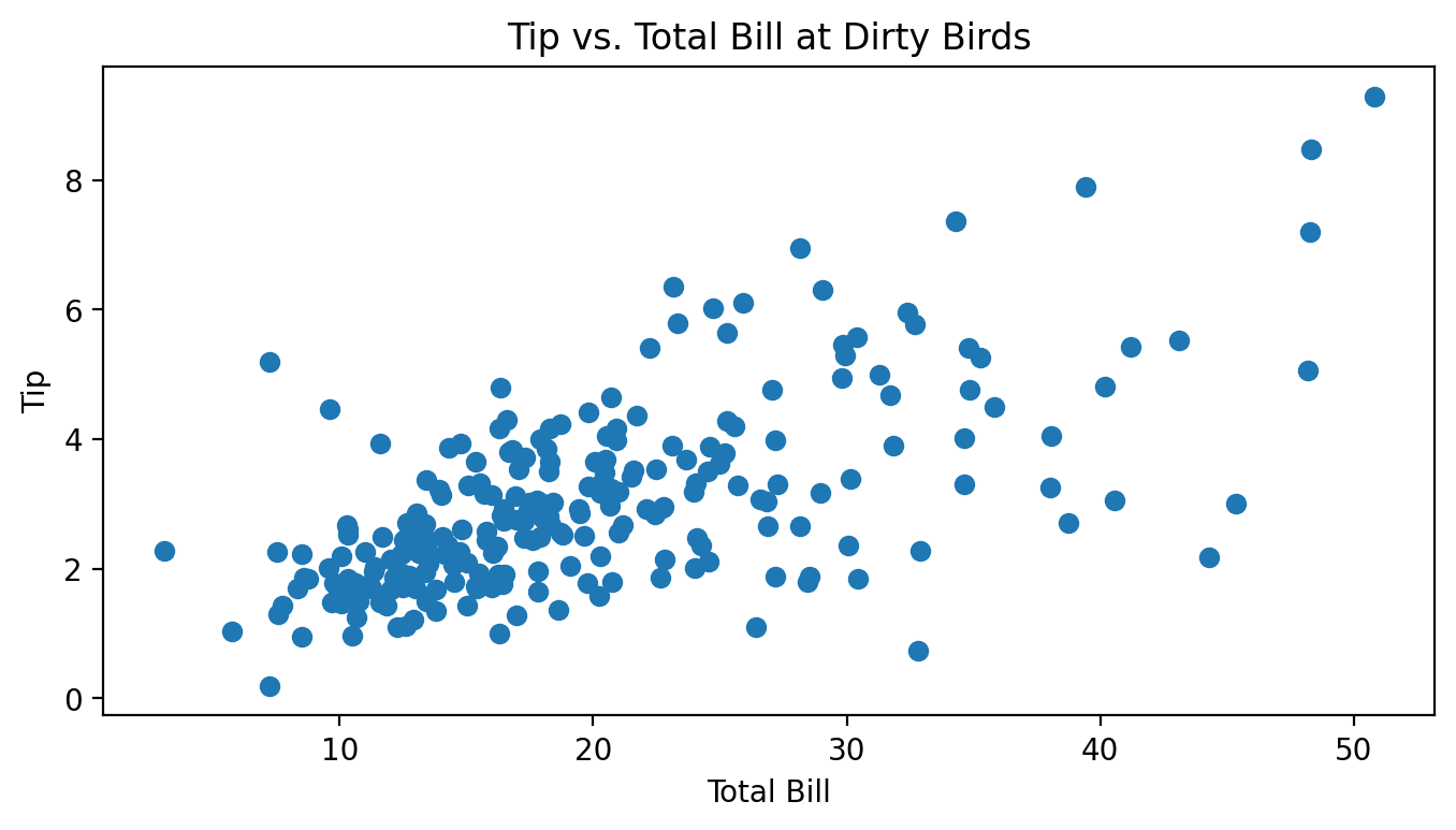
Billy decides to take on a part-time job as a waiter at the Panda Express in Pierpont. For two months, he kept track of all of the total bills he gave out to customers along with the tips they then gave him, all in dollars. Below is a scatter plot of Billy’s tips and total bills.
Throughout this question, assume we are trying to fit a linear prediction rule H(x) = w_0 + w_1x that uses total bills to predict tips, and assume we are finding optimal parameters by minimizing mean squared error.
Which of these is the most likely value for r, the correlation between total bill and tips? Why?
-1 \qquad -0.75 \qquad -0.25 \qquad 0 \qquad 0.25 \qquad 0.75 \qquad 1
0.75.
It seems like there is a pretty strong, but not perfect, linear association between total bills and tips.
The variance of the tip amounts is 2.1. Let M be the mean squared error of the best linear prediction rule on this dataset (under squared loss). Is M less than, equal to, or greater than 2.1? How can you tell?
M is less than 2.1. The variance is equal to the MSE of the constant prediction rule.
Note that the MSE of the best linear prediction rule will always be less than or equal to the MSE of the best constant prediction rule h. The only case in which these two MSEs are the same is when the best linear prediction rule is a flat line with slope 0, which is the same as a constant prediction. In all other cases, the linear prediction rule will make better predictions and hence have a lower MSE than the constant prediction rule.
In this case, the best linear prediction rule is clearly not flat, so M < 2.1.
Suppose we use the formulas from class on Billy’s dataset and calculate the optimal slope w_1^* and intercept w_0^* for this prediction rule.
Suppose we add the value of 1 to every total bill x, effectively shifting the scatter plot 1 unit to the right. Note that doing this does not change the value of w_1^*. What amount should we add to each tip y so that the value of w_0^* also does not change? Your answer should involve one or more of \bar{x}, \bar{y}, w_0^*, w_1^*, and any constants.
Note: To receive full points, you must provide a rigorous explanation, though this explanation only takes a few lines. However, we will award partial credit to solutions with the correct answer, and it’s possible to arrive at the correct answer by drawing a picture and thinking intuitively about what happens.
We should add w_1^* to each tip y.
First, we present the rigorous solution.
Let \bar{x}_\text{old} represent the previous mean of the x’s and \bar{x}_\text{new} represent the new mean of the x’s. Then, we know that \bar{x}_\text{new} = \bar{x}_\text{old} + 1.
Also, let \bar{y}_\text{old} and \bar{y}_\text{new} represent the old and new mean of the y’s. We will try and find a relationship between these two quantities.
We want the two intercepts to be the same. The intercept for the old line is \bar{y}_\text{old} - w_1^* \bar{x}_\text{old} and the intercept for the new line is \bar{y}_\text{new} - w_1^* \bar{x}_\text{new}. Setting these equal yields
\begin{aligned} \bar{y}_\text{new} - w_1^* \bar{x}_\text{new} &= \bar{y}_\text{old} - w_1^* \bar{x}_\text{old} \\ \bar{y}_\text{new} - w_1^* (\bar{x}_\text{old} + 1) &= \bar{y}_\text{old} - w_1^* \bar{x}_\text{old} \\ \bar{y}_\text{new} &= \bar{y}_\text{old} - w_1^* \bar{x}_\text{old} + w_1^* (\bar{x}_\text{old} + 1) \\ \bar{y}_{\text{new}} &= \bar{y}_\text{old} + w_1^* \end{aligned}
Thus, in order for the intercepts to be equal, we need the mean of the new y’s to be w_1^* greater than the mean of the old y’s. Since we’re told we’re adding the same constant to each y that constant is w_1^*.
Another way to approach the question is as follows: consider any point that lies directly on a line with slope w_1^* and intercept w_0^*. Consider how the slope between two points on a line is calculated: \text{slope} = \frac{y_2 - y_1}{x_2 - x_1}. If x_2 - x_1 = 1, in order for the slope to remain fixed we must have that y_2 - y_1 = \text{slope}. For a concrete example, think of the line y = 5x + 2. The point (1, 7) is on the line, as is the point (1 + 1, 7 + 5) = (2, 12).
In our case, none of our points are guaranteed to be on the line defined by slope w_1^* and intercept w_0^*. Instead, we just want to be guaranteed that the points have the same regression line after being shifted. If we follow the same principle, though, and add 1 to every x and w_1^* to every y, the points’ relative positions to the line will not change (i.e. the vertical distance from each point to the line will not change), and so that will remain the line with the lowest MSE, and hence w_0^* and w_1^* won’t change.
Suppose we have a dataset of n houses that were recently sold in the Ann Arbor area. For each house, we have its square footage and most recent sale price. The correlation between square footage and price is r.
First, we minimize mean squared error to fit a linear prediction rule that uses square footage to predict price. The resulting prediction rule has an intercept of w_0^* and slope of w_1^*. In other words,
\text{predicted price} = w_0^* + w_1^* \cdot \text{square footage}
We’re now interested in minimizing mean squared error to fit a linear prediction rule that uses price to predict square footage. Suppose this new regression line has an intercept of \beta_0^* and slope of \beta_1^*.
What is \beta_1^*? Give your answer in terms of one or more of n, r, w_0^*, and w_1^*. Show your work.
\beta_1^* = \frac{r^2}{w_1^*}
Throughout this solution, let x represent square footage and y represent price.
We know that w_1^* = r \frac{\sigma_y}{\sigma_x}. But what about \beta_1^*?
When we take a rule that predicts price from square footage and transform it into a rule that predicts square footage from price, the roles of x and y have swapped; suddenly, square footage is no longer our independent variable, but our dependent variable, and vice versa for price. This means that the altered dataset we work with when using our new prediction rule has \sigma_x standard deviation for its dependent variable (square footage), and \sigma_y for its independent variable (price). So, we can write the formula for \beta_1^* as follows: \beta_1^* = r \frac{\sigma_x}{\sigma_y}
In essence, swapping the independent and dependent variables of a dataset changes the slope of the regression line from r \frac{\sigma_y}{\sigma_x} to r \frac{\sigma_x}{\sigma_y}.
From here, we can use a little algebra to get our \beta_1^* in terms of one or more n, r, w_0^*, and w_1^*:
\begin{align*} \beta_1^* &= r \frac{\sigma_x}{\sigma_y} \\ w_1^* \cdot \beta_1^* &= w_1^* \cdot r \frac{\sigma_x}{\sigma_y} \\ w_1^* \cdot \beta_1^* &= ( r \frac{\sigma_y}{\sigma_x}) \cdot r \frac{\sigma_x}{\sigma_y} \end{align*}
The fractions \frac{\sigma_y}{\sigma_x} and \frac{\sigma_x}{\sigma_y} cancel out and we get:
\begin{align*} w_1^* \cdot \beta_1^* &= r^2 \\ \beta_1^* &= \frac{r^2}{w_1^*} \end{align*}
For this part only, assume that the following quantities hold:
Given this information, what is \beta_0^*? Give your answer as a constant, rounded to two decimal places. Show your work.
\beta_0^* = 1278.56
We start with the formula for the intercept of the regression line. Note that x and y are opposite what they’d normally be since we’re using price to predict square footage.
\beta_0^* = \bar{x} - \beta_1^* \bar{y}
We’re told that the average square footage of homes in the dataset is 2000, so \bar{x} = 2000. We also know from part (a) that \beta_1^* = \frac{r^2}{w_1^*}, and from the information given in this part this is \beta_1^* = \frac{r^2}{w_1^*} = \frac{0.6^2}{250}.
Finally, we need the average price of all homes in the dataset, \bar{y}. We aren’t given this information directly, but we can use the fact that (\bar{x}, \bar{y}) are on the regression line that uses square footage to predict price to find \bar{y}. Specifically, we have that \bar{y} = w_0^* + w_1^* \bar{x}; we know that w_0^* = 1000, \bar{x} = 2000, and w_1^* = 250, so \bar{y} = 1000 + 2000 \cdot 250 = 501000.
Putting these pieces together, we have
\begin{align*} \beta_0^* &= \bar{x} - \beta_1^* \bar{y} \\ &= 2000 - \frac{0.6^2}{250} \cdot 501000 \\ &= 2000 - 0.6^2 \cdot 2004 \\ &= 1278.56 \end{align*}
The mean of 12 non-negative numbers is 45. Suppose we remove 2 of these numbers. What is the largest possible value of the mean of the remaining 10 numbers? Show your work.
54.
To maximize the mean of the remaining 10 numbers, we want to minimize the numbers that are removed. The smallest possible non-negative number is 0, so to maximize the mean of the remaining 10, we should remove two 0s from the set of numbers. Recall that the sum of the 12 number set is 12 \cdot 45; then, the maximum possible mean of the remaining 10 is
\frac{12 \cdot 45 - 2 \cdot 0}{10} = \frac{6}{5} \cdot 45 = 54
Let R_{sq}(h) represent the mean squared error of a constant prediction h for a given dataset. Find a dataset \{y_1, y_2\} such that the graph of R_{sq}(h) has its minimum at the point (7,16).
The dataset is {3, 11}.
We’ve already learned that R_{sq}(h) is minimized at the mean of the data, and the minimum value of R_sq(h) is the variance of the data. So we need to provide a dataset of two points with a mean of 7 and a variance of 16. Recall that the variance is the average squared distance of each data point to the mean. Since we want a variance of 16, we can make each point 4 units away from the mean. Therefore, our data set can be y_1 = 3, y_2 = 11. In fact, this is the only solution.
A more calculative approach uses the formulas for mean and variance and solves a system of two equations:
\begin{aligned} \frac{y_1+y_2}{2} &= 7 \\ \frac12 \left((y_1 - 7)^2 + (y_2 - 7)^2 \right) &= 16 \end{aligned}
Consider a dataset D with 5 data points \{7,5,1,2,a\}, where a is a positive real number. Note that a is not necessarily an integer.
Express the mean of D as a function of a, simplify the expression as much as possible.
\text{Mean($D$)} = \frac{a}{5} + 3
Depending on the range of a, the median of D could assume one of three possible values. Write out all possible median of D along with the corresponding range of a for each case. Express the ranges using double inequalities, e.g., i.e. 3<a\leq8:
\begin{cases} \text{Median($D$)} = 2 & \text{if a is in the range of } 0<a\leq2 \\ \text{Median($D$)} = a & \text{if a is in the range of } 2<a\leq5 \\ \text{Median($D$)} = 5 & \text{if a is in the range of } 5<a\leq\infty \\ \end{cases}
Determine the range of a that satisfies: \text{Mean}(D) < \text{Median}(D) Make sure to show your work.
\dfrac{15}{4}<a<10
Since there are 3 possible median
values, we will have to discuss each situation separately.
In case 1, when 0<a\leq2, \text{Median}(D) = 2. So, we have:
\begin{align*} \text{Mean}(D) &< \text{Median}(D)\\ 3 + \frac{a}{5} &< 2\\ a&<-5 \end{align*}
But a<-5 is in conflict with the condition 0<a\leq2, therefore there is no solution in this situation, and Median(D) = 2 is impossible.
In case 2, when 2<a<5, \text{Median}(D) = a. So, we have:
\begin{align*} \text{Mean}(D) &< \text{Median}(D)\\ 3 + \frac{a}{5} &< a\\ 3 &< \frac{4}{5} a\\ a &> \frac{15}{4}\\ \end{align*}
So a has to be larger than \frac{15}{4}. But remember from the prerequisite condition that 2<a<5.
To satisfy both conditions, we must have \frac{15}{4}<a<5.
In case 3, when a\geq5, \text{Median}(D) = 5. So, we have:
\begin{align*} \text{Mean}(D) &< \text{Median}(D)\\ 3 + \frac{a}{5} &< 5\\ a&<10 \end{align*}
combining with the prerequisite condition, we have 5\leq a<10
Combining the range of all three cases, we have \dfrac{15}{4}<a<10 as our final answer.
Consider a dataset of n integers, y_1, y_2, ..., y_n, whose histogram is given below:
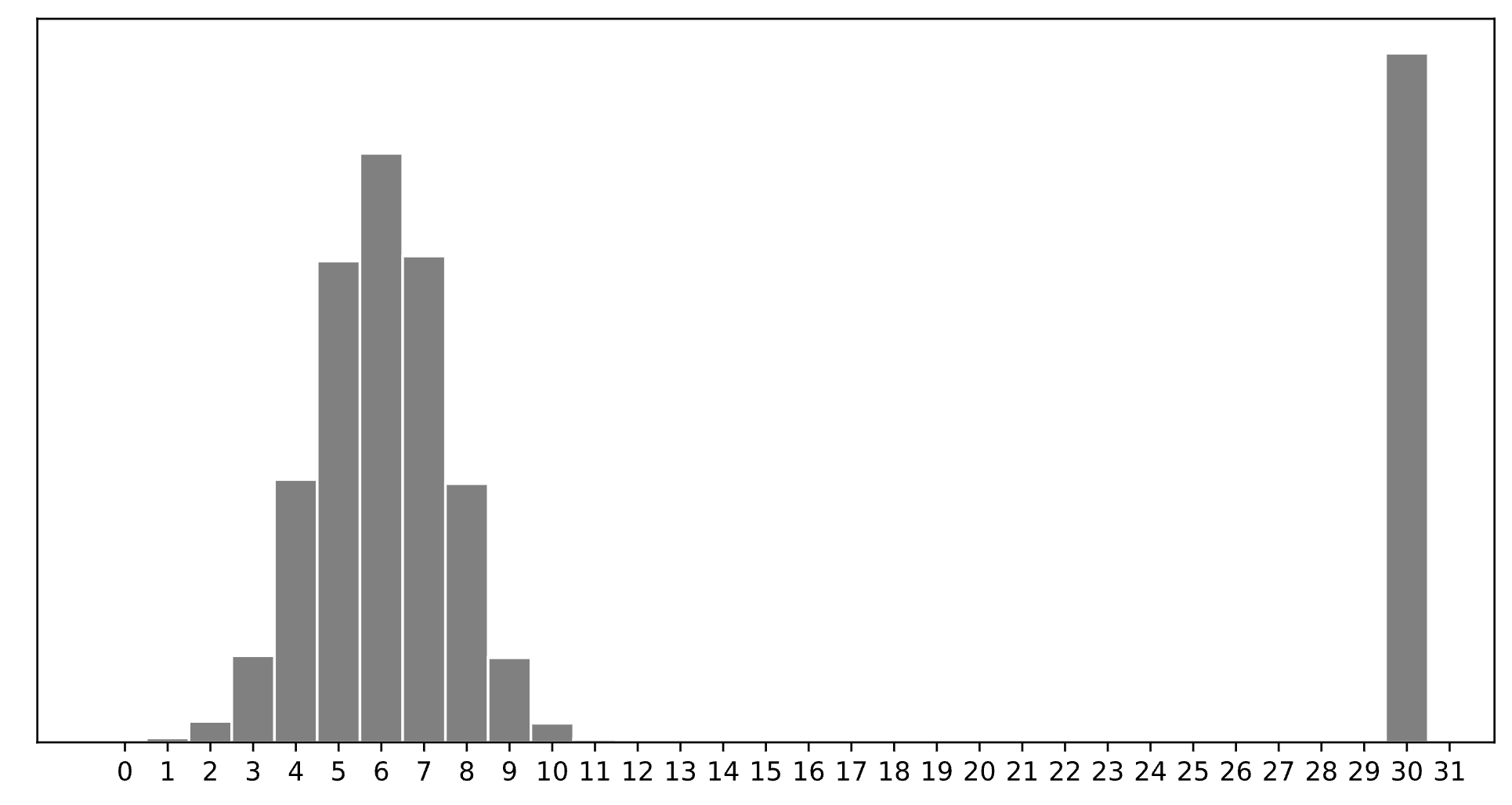
Which of the following is closest to the constant prediction h^* that minimizes:
\displaystyle \frac{1}{n} \sum_{i = 1}^n \begin{cases} 0 & y_i = h \\ 1 & y_i \neq h \end{cases}
1
5
6
7
11
15
30
30.
The minimizer of empirical risk for the constant model when using zero-one loss is the mode.
Which of the following is closest to the constant prediction h^* that minimizes: \displaystyle \frac{1}{n} \sum_{i = 1}^n |y_i - h|
1
5
6
7
11
15
30
7.
The minimizer of empirical risk for the constant model when using absolute loss is the median. If the bar at 30 wasn’t there, the median would be 6, but the existence of that bar drags the “halfway” point up slightly, to 7.
Which of the following is closest to the constant prediction h^* that minimizes: \displaystyle \frac{1}{n} \sum_{i = 1}^n (y_i - h)^2
1
5
6
7
11
15
30
11.
The minimizer of empirical risk for the constant model when using squared loss is the mean. The mean is heavily influenced by the presence of outliers, of which there are many at 30, dragging the mean up to 11. While you can’t calculate the mean here, given the large right tail, this question can be answered by understanding that the mean must be larger than the median, which is 7, and 11 is the next biggest option.
Which of the following is closest to the constant prediction h^* that minimizes: \displaystyle \lim_{p \rightarrow \infty} \frac{1}{n} \sum_{i = 1}^n |y_i - h|^p
1
5
6
7
11
15
30
15.
The minimizer of empirical risk for the constant model when using infinity loss is the midrange, i.e. halfway between the min and max.
Suppose there is a dataset containing 10000 integers:
Calculate the median of this dataset.
6
We know there is an even number of integers in this dataset because 10000 \% 2 = 0. We can find the middle of the dataset as follows: \frac{10000}{2} = 5000. This means the element in the 5000th position and 5001st position can give us our median. The element at the 5000th position is a 5 because 2500 + 2500 = 5000. The element at the 5001st position is a 7 because the next number after 5 is 7. We can then plug 5 and 7 into the equation: \frac{x_{5000} + x_{5001}}{2} = \frac{5 + 7}{2} = 6
How does the mean of this dataset compared to its median?
The mean is larger than the median
The mean is smaller than the median
The mean and the median are equal
The mean is smaller than the median.
We can calculate the mean as follows: \frac{2500 \cdot 3 + 2500 \cdot 5 + 4500 \cdot 7 + 500 \cdot 9}{10000} = 5.6 Using part (a) we know that 5.6 < 6, which means the mean is smaller than the median.
Define the extreme mean (EM) of a dataset to be the average of its largest and smallest values. Let f(x)=-3x+4. Show that for any dataset x_1\leq x_2 \leq \dots \leq x_n, EM(f(x_1), f(x_2), \dots, f(x_n)) = f(EM(x_1, x_2, \dots, x_n)).
This linear transformation reverses the order of the data because if a<b, then -3a>-3b and so adding four to both sides gives f(a)>f(b). Since x_1\leq x_2 \leq \dots \leq x_n, this means that the smallest of f(x_1), f(x_2), \dots, f(x_n) is f(x_n) and the largest is f(x_1). Therefore,
\begin{aligned} EM(f(x_1), f(x_2), \dots, f(x_n)) &= \dfrac{f(x_n) + f(x_1)}{2} \\ &= \dfrac{-3x_n+4-3x_1+4}{2} \\ &= \dfrac{-3x_n-3x_1}{2} + 4\\ &= -3\left(\dfrac{x_1+x_n}{2}\right) + 4 \\ &= -3EM(x_1, x_2, \dots, x_n)+ 4\\ &= f(EM(x_1, x_2, \dots, x_n)). \end{aligned}
Consider a dataset of n values, y_1, y_2, ..., y_n, all of which are non-negative. We’re interested in fitting a constant model, H(x) = h, to the data, using the new “Wolverine” loss function:
L_\text{wolverine}(y_i, h) = w_i \left( y_i^2 - h^2 \right)^2
Here, w_i corresponds to the “weight” assigned to the data point y_i, the idea being that different data points can be weighted differently when finding the optimal constant prediction, h^*.
For example, for the dataset y_1 = 1, y_2 = 5, y_3 = 2, we will end up with different values of h^* when we use the weights w_1 = w_2 = w_3 = 1 and when we use weights w_1 = 8, w_2 = 4, w_3 = 3.
Find \frac{\partial L_\text{wolverine}}{\partial h}, the derivative of the Wolverine loss function with respect to h. Show your work.
\frac{\partial L}{\partial h} = -4w_ih(y_i^2 -h^2)
To solve this problem we simply take the derivative of L_\text{wolverine}(y_i, h) = w_i( y_i^2 - h^2 )^2.
We can use the chain rule to find the derivative. The chain rule is: \frac{\partial}{\partial h}[f(g(h))]=f'(g(h))g'(h).
Note that (y_i^2 -h^2)^2 is the area we care about inside of L_\text{wolverine}(y_i, h) = w_i( y_i^2 - h^2 )^2 because that is where h is!. In this case f(h) = h^2 and g(h) = y_i^2 - h^2. We can then take the derivative of both to get: f'(h) = 2h and g'(x) = -2h.
This tells us the derivative is: \frac{\partial L}{\partial h} = (w_i) * 2(y_i^2 -h^2) * (-2h), which can be simplified to \frac{\partial L}{\partial h} = -4w_ih(y_i^2 -h^2).
Prove that the constant prediction that minimizes average loss for the Wolverine loss function is:
h^* = \sqrt{\frac{\sum_{i = 1}^n w_i y_i^2}{\sum_{i = 1}^n w_i}}
The recipe for average loss is to find the derivative of the risk function, set it equal to zero, and solve for h^*.
We know that average loss follows the equation R(L(y_i, h)) = \frac{1}{n} \sum_{i=1}^n L(y_i, h). This means that R_\text{wolverine}(h) = \frac{1}{n} \sum_{i = 1}^n w_i (y_i^2 - h^2)^2.
Recall we have already found the derivative of L_\text{wolverine}(y_i, h) = w_i ( y_i^2 - h^2)^2. Which means that \frac{\partial R}{\partial h}(h) = \frac{1}{n} \sum_{i = 1}^n \frac{\partial L}{\partial h}(h). So we can set \frac{\partial}{\partial h}(h) R_\text{wolverine}(h) = \frac{1}{n} \sum_{i = 1}^n -4hw_i(y_i^2 -h^2).
We can now do the last two steps: \begin{align*} 0 &= \frac{1}{n} \sum_{i = 1}^n -4hw_i(y_i^2 -h^2)\\ 0&= \frac{-4h}{n} \sum_{i = 1}^n w_ih(y_i^2 -h^2)\\ 0&= \sum_{i = 1}^n w_i(y_i^2 -h^2)\\ 0&= \sum_{i = 1}^n w_iy_i^2 -w_ih^2\\ 0&= \sum_{i = 1}^n w_iy_i^2 - \sum_{i = 1}^n w_ih^2\\ \sum_{i = 1}^n w_ih^2 &= \sum_{i = 1}^n w_iy_i^2\\ h^2\sum_{i = 1}^n w_i &= \sum_{i = 1}^n w_iy_i^2\\ h^2 &= \frac{\sum_{i = 1}^n w_iy_i^2}{\sum_{i = 1}^n w_i}\\ h^* &= \sqrt{\frac{\sum_{i = 1}^n w_iy_i^2}{\sum_{i = 1}^n w_i}} \end{align*}
For a dataset of non-negative values y_1, y_2, ..., y_n with weights w_1, 1, ..., 1, evaluate: \displaystyle \lim_{w_1 \rightarrow \infty} h^*
The maximum of y_1, y_2, ..., y_n
The mean of y_1, y_2, ..., y_{n-1}
The mean of y_2, y_3, ..., y_n
The mean of y_2, y_3, ..., y_n, multiplied by \frac{n}{n-1}
y_1
y_n
y_1
Recall from part b h^* = \sqrt{\frac{\sum_{i = 1}^n w_i y_i^2}{\sum_{i = 1}^n w_i}}.
The problem is asking us \lim_{w_1 \rightarrow \infty} \sqrt{\frac{\sum_{i = 1}^n w_i y_i^2}{\sum_{i = 1}^n w_i}}.
We can further rewrite the problem to get something like this: \lim_{w_1 \rightarrow \infty} \sqrt{\frac{w_1 y_1^2 + \sum_{i=1}^{n-1}y_i^2}{w_1 + (n-1)}}. Note that \frac{\sum_{i=1}^{n-1}y_i^2}{n-1} is insignificant because it is a constant. Constants compared to infinity can be ignored. We now have something like \sqrt{\frac{w_1y_1^2}{w_1}}. We can cancel out the w_1 to get \sqrt{y_1^2}, which becomes y_1.
Suppose we’re given a dataset of n points, (x_1, y_1), (x_2, y_2), ..., (x_n, y_n), where \bar{x} is the mean of x_1, x_2, ..., x_n and \bar{y} is the mean of y_1, y_2, ..., y_n.
Using this dataset, we create a transformed dataset of n points, (x_1', y_1'), (x_2', y_2'), ..., (x_n', y_n'), where:
x_i' = 4x_i - 3 \qquad y_i' = y_i + 24
That is, the transformed dataset is of the form (4x_1 - 3, y_1 + 24), ..., (4x_n - 3, y_n + 24).
We decide to fit a simple linear hypothesis function H(x') = w_0 + w_1x' on the transformed dataset using squared loss. We find that w_0^* = 7 and w_1^* = 2, so H^*(x') = 7 + 2x'.
Suppose we were to fit a simple linear hypothesis function through the original dataset, (x_1, y_1), (x_2, y_2), ..., (x_n, y_n), again using squared loss. What would the optimal slope be?
2
4
6
8
11
12
24
8.
Relative to the dataset with x', the dataset with x has an x-variable that’s “compressed” by a factor of 4, so the slope increases by a factor of 4 to 2 \cdot 4 = 8.
Concretely, this can be shown by looking at the formula 2 = r\frac{SD(y')}{SD(x')}, recognizing that SD(y') = SD(y) since the y values have the same spread in both datasets, and that SD(x') = 4 SD(x).
Recall, the hypothesis function H^* was fit on the transformed dataset,
(x_1', y_1'), (x_2', y_2'), ..., (x_n', y_n'). H^* happens to pass through the point (\bar{x}, \bar{y}). What is the value of \bar{x}? Give your answer as an integer with no variables.
5.
The key idea is that the regression line always passes through (\text{mean } x, \text{mean } y) in the dataset we used to fit it. So, we know that: 2 \bar{x'} + 7 = \bar{y'}. This first equation can be rewritten as: 2 \cdot (4\bar{x} - 3) + 7 = \bar{y} + 24.
We’re also told this line passes through (\bar{x}, \bar{y}), which means that it’s also true that: 2 \bar{x} + 7 = \bar{y}.
Now we have a system of two equations:
\begin{cases} 2 \cdot (4\bar{x} - 3) + 7 = \bar{y} + 24 \\ 2 \bar{x} + 7 = \bar{y} \end{cases}
\dots and solving our system of two equations gives: \bar{x} = 5.
For a given dataset \{y_1, y_2, \dots, y_n\}, let M_{abs}(h) represent the median absolute error of the constant prediction h on that dataset (as opposed to the mean absolute error R_{abs}(h)).
For the dataset \{4, 9, 10, 14, 15\}, what is M_{abs}(9)?
5
The first step is to calculate the absolute errors (|y_i - h|).
\begin{align*} \text{Absolute Errors} &= \{|4-9|, |9-9|, |10-9|, |14-9|, |15-9|\} \\ \text{Absolute Errors} &= \{|-5|, |0|, |1|, |5|, |6|\} \\ \text{Absolute Errors} &= \{5, 0, 1, 5, 6\} \end{align*}
Now we have to order the values inside of the absolute errors: \{0, 1, 5, 5, 6\}. We can see the median is 5, so M_{abs}(9) =5.
For the same dataset \{4, 9, 10, 14, 15\}, find another integer h such that M_{abs}(9) = M_{abs}(h).
5 or 15
Our goal is to find another number that will give us the same median of absolute errors as in part (a).
One way to do this is to plug in a number and guess. Another way requires noticing you can modify 10 (the middle element) to become 5 in either direction (negative or positive) because of the absolute value.
We can solve this equation to get |10-x| = 5 \rightarrow x = 15 \text{ and } x = 5.
We can then test this by following the same steps as we did in part (a).
For x = 15:
\begin{align*} \text{Absolute Errors} &= \{|4-15|, |9-15|, |10-15|, |14-15|, |15-15|\} \\ \text{Absolute Errors} &= \{|-11|, |-6|, |-5|, |-1|, |0|\} \\ \text{Absolute Errors} &= \{11, 6, 5, 1, 0\} \end{align*}
Then we order the elements to get the absolute errors: \{0, 1, 5, 6, 11\}. We can see the median is 5, so M_{abs}(15) =5.
For x = 5:
\begin{align*} \text{Absolute Errors} &= \{|4-5|, |9-5|, |10-5|, |14-5|, |15-5|\} \\ \text{Absolute Errors} &= \{|-1|, |4|, |5|, |9|, |10|\} \\ \text{Absolute Errors} &= \{1, 4, 5, 9, 10\} \end{align*}
We do not have to re-order the elements because they are in order already. We can see the median is 5, so M_{abs}(5) =5.
Based on your answers to parts (a) and (b), discuss in at most two sentences what is problematic about using the median absolute error to make predictions.
The numbers 5 and 15 are clearly bad predictions (close to the extreme values in the dataset), yet they are considered just as good a prediction by this metric as the number 9, which is roughly in the center of the dataset. Intuitively, 9 is a much better prediction, but this way of measuring the quality of a prediction does not recognize that.
Suppose we are given a dataset of points \{(x_1, y_1), (x_2, y_2), \dots, (x_n, y_n)\} and for some reason, we want to make predictions using a prediction rule of the form H(x) = 17 + w_1x.
Write down an expression for the mean squared error of a prediction rule of this form, as a function of the parameter w_1.
MSE(w_1) = \dfrac1n \displaystyle\sum_{i=1}^n (y_i - (17 + w_1x_i))^2
Minimize the function MSE(w_1) to find the parameter w_1^* which defines the optimal prediction rule H^*(x) = 17 + w_1^*x. Show all your work and explain your steps.
Fill in your final answer below:
w_1^* = \dfrac{\displaystyle\sum_{i=1}^n x_i(y_i - 17)}{\displaystyle\sum_{i=1}^n x_i^2}
To minimize a function of one variable, we need to take the derivative, set it equal to zero, and solve. \begin{aligned} MSE(w_1) &= \dfrac1n \displaystyle\sum_{i=1}^n (y_i - 17 - w_1x_i)^2 \\ MSE'(w_1) &= \dfrac1n \displaystyle\sum_{i=1}^n -2x_i(y_i - 17 - w_1x_i)) \qquad \text{using the chain rule} \\ 0 &= \dfrac1n \displaystyle\sum_{i=1}^n -2x_i(y_i - 17) + \dfrac1n \displaystyle\sum_{i=1}^n 2x_i^2w_1 \qquad \text{splitting up the sum} \\ 0 &= \displaystyle\sum_{i=1}^n -x_i(y_i - 17) + \displaystyle\sum_{i=1}^n x_i^2w_1 \qquad \text{multiplying through by } \frac{n}{2} \\ w_1 \displaystyle\sum_{i=1}^n x_i^2 &= \displaystyle\sum_{i=1}^n x_i(y_i - 17) \qquad \text{rearranging terms and pulling out } w_1 \\ w_1 & = \dfrac{\displaystyle\sum_{i=1}^n x_i(y_i - 17)}{\displaystyle\sum_{i=1}^n x_i^2} \end{aligned}
True or False: For an arbitrary dataset, the prediction rule H^*(x) = 17 + w_1^*x goes through the point (\bar x, \bar y).
True
False
False.
When we fit a prediction rule of the form H(x) = w_0+w_1x using simple linear regression, the formula for the intercept w_0 is designed to make sure the regression line passes through the point (\bar x, \bar y). Here, we don’t have the freedom to control our intercept, as it’s forced to be 17. This means we can’t guarantee that the prediction rule H^*(x) = 17 + w_1^*x goes through the point (\bar x, \bar y).
A simple example shows that this is the case. Consider the dataset (-2, 0) and (2, 0). The point (\bar x, \bar y) is the origin, but the prediction rule H^*(x) does not pass through the origin because it has an intercept of 17.
True or False: For an arbitrary dataset, the mean squared error associated with H^*(x) is greater than or equal to the mean squared error associated with the regression line.
True
False
True.
The regression line is the prediction rule of the form H(x) = w_0+w_1x with the smallest mean squared error (MSE). H^*(x) is one example of a prediction rule of that form so unless it happens to be the regression line itself, the regression line will have lower MSE because it was designed to have the lowest possible MSE. This means the MSE associated with H^*(x) is greater than or equal to the MSE associated with the regression line.
Suppose you have a dataset \{(x_1, y_1), (x_2,y_2), \dots, (x_8, y_8)\} with n=8 ordered pairs such that the variance of \{x_1, x_2, \dots, x_8\} is 50. Let m be the slope of the regression line fit to this data.
Suppose now we fit a regression line to the dataset \{(x_1, y_2), (x_2,y_1), \dots, (x_8, y_8)\} where the first two y-values have been swapped. Let m' be the slope of this new regression line.
If x_1 = 3, y_1 =7, x_2=8, and y_2=2, what is the difference between the new slope and the old slope? That is, what is m' - m? The answer you get should be a number with no variables.
Hint: There are many equivalent formulas for the slope of the regression line. We recommend using the version of the formula without \overline{y}.
m' - m = \dfrac{1}{16}
Using the formula for the slope of the regression line, we have:
\begin{aligned} m &= \frac{\sum_{i=1}^n (x_i - \overline x)y_i}{\sum_{i=1}^n (x_i - \overline x)^2}\\ &= \frac{\sum_{i=1}^n (x_i - \overline x)y_i}{n\cdot \sigma_x^2}\\ &= \frac{(3-\bar{x})\cdot 7 + (8 - \bar{x})\cdot 2 + \sum_{i=3}^n (x_i - \overline x)y_i}{8\cdot 50}. \\ \end{aligned}
Note that by switching the first two y-values, the terms in the sum from i=3 to n, the number of data points n, and the variance of the x-values are all unchanged.
So the slope becomes:
\begin{aligned} m' &= \frac{(3-\bar{x})\cdot 2 + (8 - \bar{x})\cdot 7 + \sum_{i=3}^n (x_i - \overline x)y_i}{8\cdot 50} \\ \end{aligned}
and the difference between these slopes is given by:
\begin{aligned} m'-m &= \frac{(3-\bar{x})\cdot 2 + (8 - \bar{x})\cdot 7 - ((3-\bar{x})\cdot 7 + (8 - \bar{x})\cdot 2)}{8\cdot 50}\\ &= \frac{(3-\bar{x})\cdot 2 + (8 - \bar{x})\cdot 7 - (3-\bar{x})\cdot 7 - (8 - \bar{x})\cdot 2}{8\cdot 50}\\ &= \frac{(3-\bar{x})\cdot (-5) + (8 - \bar{x})\cdot 5}{8\cdot 50}\\ &= \frac{ -15+5\bar{x} + 40 -5\bar{x}}{8\cdot 50}\\ &= \frac{ 25}{8\cdot 50}\\ &= \frac{ 1}{16} \end{aligned}
Note that we have two simplified closed form expressions for the estimated slope w in simple linear regression that you have already seen in discussions and lectures:
\begin{align*} w &= \frac{\sum_i (x_i - \overline{x}) y_i}{\sum_i (x_i - \overline{x})^2} \\ \\ w &= \frac{\sum_i (y_i - \overline{y}) x_i }{\sum_i (x_i - \overline{x})^2} \end{align*}
where we have dataset D = [(x_1,y_1), \ldots, (x_n,y_n)] and sample means \overline{x} = {1 \over n} \sum_{i} x_i, \quad \overline{y} = {1 \over n} \sum_{i} y_i. Without further explanation, \sum_i means \sum_{i=1}^n
Are (1) and (2) equivalent? That is, is the following equality true? Prove or disprove it. \sum_i (x_i - \overline{x}) y_i = \sum_i (y_i - \overline{y}) x_i
True.
\begin{align*} & \sum_i (x_i - \overline{x}) y_i = \sum_i (y_i - \overline{y}) x_i \\ & \Leftrightarrow \sum_i x_i y_i - \overline{x} \sum_i y_i = \sum_i x_i y_i - \overline{y} \sum_i x_i \\ & \Leftrightarrow \overline{x} \sum_i y_i = \overline{y} \sum_i x_i \\ & \Leftrightarrow {1 \over n} \sum_i x_i \sum_i y_i = {1 \over n} \sum_i y_i \sum_i x_i \\ \end{align*}
True or False: If the dataset shifted right by a constant distance a, that is, we have the new dataset D_a = (x_1 + a,y_1), \ldots, (x_n + a,y_n), then will the estimated slope w change or not?
True
False
False. By (1) in part (a), we can view w as only being affected by x_i - \overline{x}, which is unchanged after shifting horizontally. Therefore, w is unchanged.
True or False: If the dataset shifted up by a constant distance b, that is, we have the new dataset D_b = [(x_1,y_1 + b), \ldots, (x_n,y_n + b)], then will the estimated slope w change or not?
True
False
False. By (2) in part (a), we can view w as only being affected by y_i - \overline{y}, which is unchanged after shifting vertically. Therefore, w is unchanged.
Consider a dataset that consists of y_1, \cdots, y_n. In class, we used calculus to minimize mean squared error, R_{sq}(h) = \frac{1}{n} \sum_{i = 1}^n (h - y_i)^2. In this problem, we want you to apply the same approach to a slightly different loss function defined below: L_{\text{midterm}}(y,h)=(\alpha y - h)^2+\lambda h
Write down the empiricial risk R_{\text{midterm}}(h) by using the above loss function.
R_{\text{midterm}}(h)=\frac{1}{n}\sum_{i=1}^{n}[(\alpha y_i - h)^2+\lambda h]=[\frac{1}{n}\sum_{i=1}^{n}(\alpha y_i - h)^2] +\lambda h
The mean of dataset is \bar{y}, i.e. \bar{y} = \frac{1}{n} \sum_{i = 1}^n y_i. Find h^* that minimizes R_{\text{midterm}}(h) using calculus. Your result should be in terms of \bar{y}, \alpha and \lambda.
h^*=\alpha \bar{y} - \frac{\lambda}{2}
\begin{align*} \frac{d}{dh}R_{\text{midterm}}(h)&= [\frac{2}{n}\sum_{i=1}^{n}(h- \alpha y_i )] +\lambda \\ &=2 h-2\alpha \bar{y} + \lambda. \end{align*}
By setting \frac{d}{dh}R_{\text{midterm}}(h)=0 we get 2 h^*-2\alpha \bar{y} + \lambda=0 \Rightarrow h^*=\alpha \bar{y} - \frac{\lambda}{2}.