← return to study.practicaldsc.org

The problems in this worksheet are taken from past exams in similar classes. Work on them on paper, since the exams you take in this course will also be on paper.

Problem 1

The laptops DataFrame contains information on various factors that influence the pricing of laptops. Each row represents a laptop, and the columns are:

• "Mfr" (str): the company that manufactures the laptop, like “Apple” or “Dell”.
• "Model" (str): the model name of the laptop, such as “MacBook Pro”.
• "OS" (str): the operating system, such as “macOS” or “Windows 11”.
• "Screen Size" (float): the diagonal length of the screen, in inches.
• "Price" (float): the price of the laptop, in dollars.

Problem 1.1

Without using groupby, write an expression that evaluates to the average price of laptops with the "macOS" operating system (the same quantity as above).

Problem 1.2

Using groupby, write an expression that evaluates to the average price of laptops with the "macOS" operating system.

Problem 2

You are given a DataFrame called books that contains columns 'author' (string), 'title' (string), 'num_chapters' (int), and 'publication_year' (int).

Suppose that after doing books.groupby('author').max(), one row says

Problem 2.1

Based on this data, can you conclude that Charles Dickens is the alphabetically last of all author names in this dataset?

• Yes

• No

Problem 2.2

Based on this data, can you conclude that Charles Dickens wrote Oliver Twist?

• Yes

• No

Problem 2.3

Based on this data, can you conclude that Oliver Twist has 53 chapters?

• Yes

• No

Problem 2.4

Based on this data, can you conclude that Charles Dickens wrote a book with 53 chapters that was published in 1838?

• Yes

• No

Problem 3

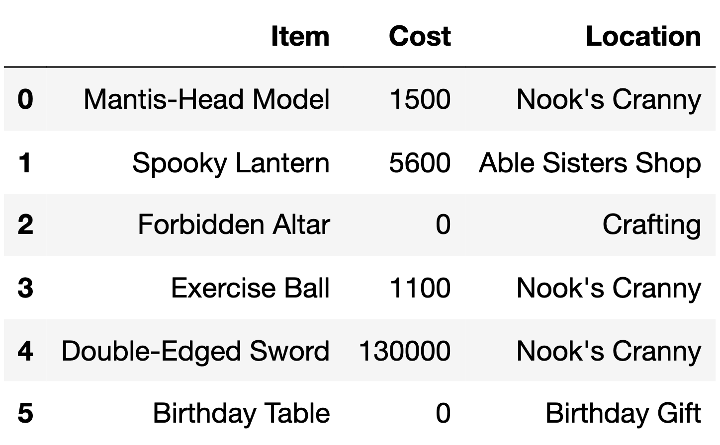
The DataFrame items describes various items available to collect or purchase using bells, the currency used in the game Animal Crossing: New Horizons.

For each item, we have:

• "Item" (str): The name of the item.
• "Cost" (int): The cost of the item in bells. Items that cost 0 bells cannot be purchased and must be collected through other means (such as crafting).
• "Location" (str): The store or action through which the item can be obtained.

The first 6 rows of items are below, though items has more rows than are shown here.

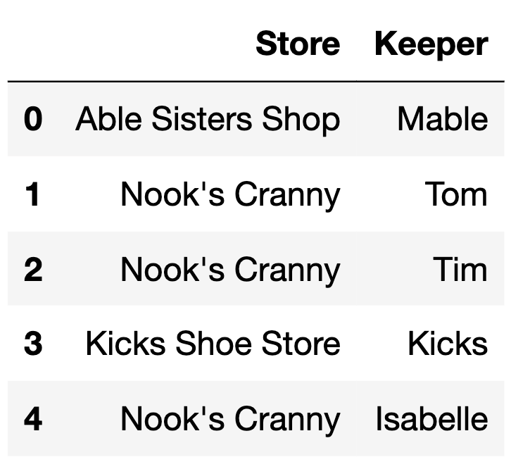
The DataFrame keepers has 5 rows, each of which represent a different shopkeeper in the Animal Crossing: New Horizons universe.

keepers is shown below in its entirety.

How many rows are in the following DataFrame? Give your answer as an integer.

keepers.merge(items.iloc[:6], 
              left_on="Store", 
              right_on="Location")

Problem 4

Suppose we create a DataFrame called midwest containing Nishant’s flights departing from DTW, ORD, and MKE. midwest has 10 rows; the bar chart below shows how many of these 10 flights departed from each airport.

Consider the DataFrame that results from merging midwest with itself, as follows:

double_merge = midwest.merge(midwest, left_on='FROM', right_on='FROM')

How many rows does double_merge have?

Problem 5

In this problem, we will be using the following DataFrame students, which contains various information about high school students and the university/universities they applied to.

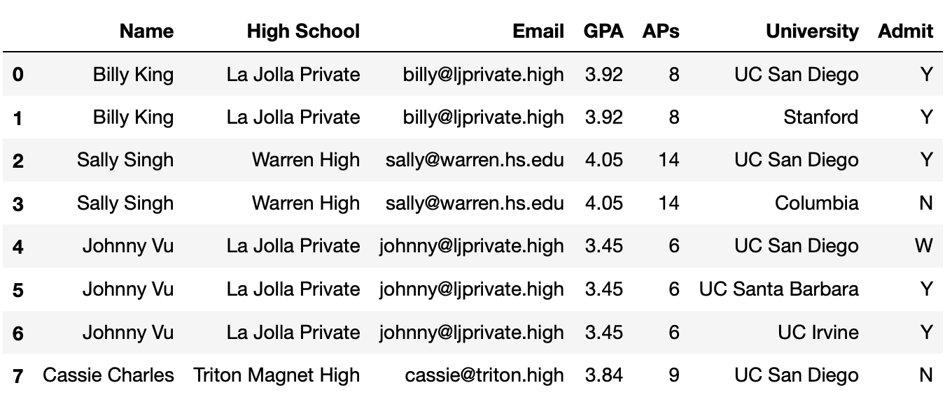
The columns are:

• 'Name' (str): the name of the student.
• 'High School' (str): the High School that the student attended.
• 'Email' (str): the email of the student.
• 'GPA' (float): the GPA of the student.
• 'AP' (int): the number of AP exams that the student took.
• 'University' (str): the name of the university that the student applied to.
• 'Admit' (str): the acceptance status of the student (where ‘Y’ denotes that they were accepted to the university, ‘N’ denotes that they were not and ‘W’ denotes that they were waitlisted).

The rows of 'student' are arranged in no particular order. The first eight rows of 'student' are shown above (though 'student' has many more rows than pictured here).

Problem 5.1

Fill in the blank so that the result evaluates to a Series indexed by "Email" that contains a list of the universities that each student was admitted to. If a student wasn’t admitted to any universities, they should have an empty list.

    students.groupby("Email").apply(_____)

What goes in the blank?

Problem 5.2

Which of the following blocks of code correctly assign max_AP to the maximum number of APs taken by a student who was rejected by UC San Diego?

Option 1:

cond1 = students["Admit"] == "N"
cond2 = students["University"] == "UC San Diego"
max_AP = students.loc[cond1 & cond2, "APs"].sort_values().iloc[-1]

Option 2:

cond1 = students["Admit"] == "N"
cond2 = students["University"] == "UC San Diego"
d3 = students.groupby(["University", "Admit"]).max().reset_index()
max_AP = d3.loc[cond1 & cond2, "APs"].iloc[0]

Option 3:

p = students.pivot_table(index="Admit", 
                            columns="University", 
                            values="APs", 
                            aggfunc="max")
max_AP = p.loc["N", "UC San Diego"]

Option 4:

# .last() returns the element at the end of a Series it is called on
groups = students.sort_values(["APs", "Admit"]).groupby("University")
max_AP = groups["APs"].last()["UC San Diego"]

Select all that apply. There is at least one correct option.

• Option 1

• Option 2

• Option 3

• Option 4

Problem 5.3

Currently, students has a lot of repeated information — for instance, if a student applied to 10 universities, their GPA appears 10 times in students.

We want to generate a DataFrame that contains a single row for each student, indexed by "Email", that contains their "Name", "High School", "GPA", and "APs".

One attempt to create such a DataFrame is below.

students.groupby("Email").aggregate({"Name": "max",
                                        "High School": "mean",
                                        "GPA": "mean",
                                        "APs": "max"})

There is exactly one issue with the line of code above. In one sentence, explain what needs to be changed about the line of code above so that the desired DataFrame is created.

Problem 5.4

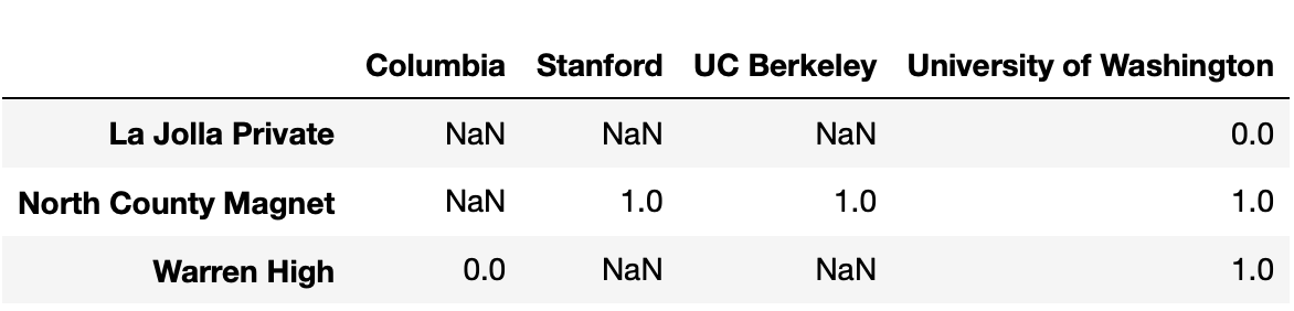
Consider the following snippet of code.

pivoted = students.assign(Admit=students["Admit"] == "Y") \
                    .pivot_table(index="High School", 
                                columns="University", 
                                values="Admit", 
                                aggfunc="sum")

Some of the rows and columns of pivoted are shown below.

No students from Warren High were admitted to Columbia or Stanford. However,
pivoted.loc["Warren High", "Columbia"] and pivoted.loc["Warren High", "Stanford"] evaluate to different values. What is the reason for this difference?

• Some students from Warren High applied to Stanford, and some others applied to Columbia, but none applied to both.

• Some students from Warren High applied to Stanford but none applied to Columbia.

• Some students from Warren High applied to Columbia but none applied to Stanford.

• The students from Warren High that applied to both Columbia and Stanford were all rejected from Stanford, but at least one was admitted to Columbia.

• When using pivot_table, pandas was not able to sum strings of the form "Y", "N", and "W", so the values in pivoted are unreliable.

Problem 6

The DataFrame dogs, contains one row for every registered pet dog in Zurich, Switzerland in 2017.

The first few rows of dogs are shown below, but dogs has many more rows than are shown.

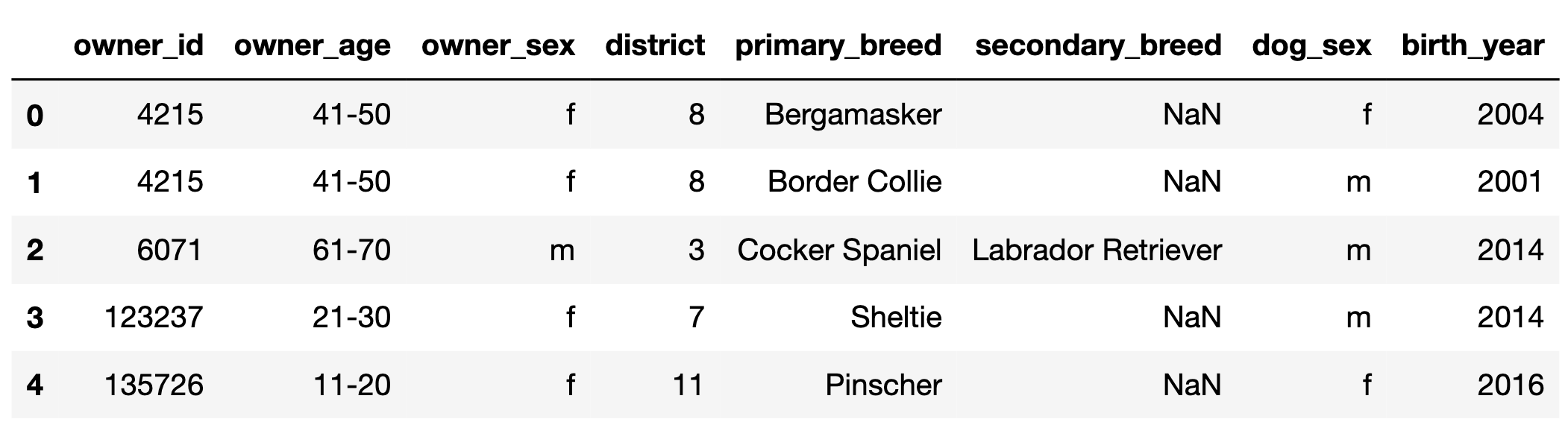
• "owner_id" (int): A unique ID for each owner. Note that, for example, there are two rows in the preview for 4215, meaning that owner has at least 2 dogs. Assume that if an "owner_id" appears in dogs multiple times, the corresponding "owner_age", "owner_sex", and "district" are always the same.
• "owner_age" (str): The age group of the owner; either "11-20", "21-30", …, or "91-100" (9 possibilities in total).
• "owner_sex" (str): The birth sex of the owner; either "m" (male) or "f" (female).
• "district" (int): The city district the owner lives in; a positive integer between 1 and 12 (inclusive).
• "primary_breed" (str): The primary breed of the dog.
• "secondary_breed" (str): The secondary breed of the dog. If this column is not null, the dog is a “mixed breed” dog; otherwise, the dog is a “purebred” dog.
• "dog_sex" (str): The birth sex of the dog; either "m" (male) or "f" (female).
• "birth_year" (int): The birth year of the dog.

In this question, assume that there are more than 12 districts in dogs.

Suppose we merge the dogs DataFrame with itself as follows.

# on="x" is the same as specifying both left_on="x" and right_on="x".
double = dogs.merge(dogs, on="district")

# sort_index sorts a Series in increasing order of its index.
square = double["district"].value_counts().value_counts().sort_index()

The first few rows of square are shown below.

1     5500
4      215
9       40

Problem 6.1

In dogs, there are 12 rows with a "district" of 8. How many rows of double have a "district" of 8? Give your answer as a positive integer.

Problem 6.2

What does the following expression evaluate to? Give your answer as a positive integer.

dogs.groupby("district").filter(lambda df: df.shape[0] == 3).shape[0]

Hint: Unlike in 6.1, your answer to 6.2 depends on the values in square.

Problem 7

Kyle and Yutong are trying to decide where they’ll study on campus and start flipping a Michigan-themed coin, with a picture of the Michigan Union on the heads side and a picture of the Shapiro Undergraduate Library (aka the UgLi) on the tails side.

Kyle flips the coin 21 times and sees 13 heads and 8 tails. He stores this information in a DataFrame named kyle that has 21 rows and 2 columns, such that:

• The "flips" column contains "Heads" 13 times and "Tails" 8 times.

• The "Markley" column contains "Kyle" 21 times.

Then, Yutong flips the coin 11 times and sees 4 heads and 7 tails. She stores this information in a DataFrame named yutong that has 11 rows and 2 columns, such that:

• The "flips" column contains "Heads" 4 times and "Tails" 7 times.

• The "MoJo" column contains "Yutong" 11 times.

Problem 7.1

How many rows are in the following DataFrame? Give your answer as an integer.

    kyle.merge(yutong, on="flips")

Hint: The answer is less than 200.

Problem 7.2

Let A be your answer to the previous part. Now, suppose that:

• kyle contains an additional row, whose "flips" value is "Total" and whose "Markley" value is 21.

• yutong contains an additional row, whose "flips" value is "Total" and whose "MoJo" value is 11.

Suppose we again merge kyle and yutong on the "flips" column. In terms of A, how many rows are in the new merged DataFrame?

• A

• A+1

• A+2

• A+4

• A+231

Problem 8

The h table records addresses within San Diego. Only 50 addresses are recorded. The index of the DataFrame contains the numbers 1-50 as unique integers.

• "number" (int): Street address number
• "street" (str): Street name

Fill in the Python code to create a DataFrame containing the proportion of 4-digit address numbers for each unique street in h.

def foo(x):
    lengths = __(a)__
    return (lengths == 4).mean()

h.groupby(__(b)__).__(c)__(foo)

Problem 9

Define small_students to be the DataFrame with 8 rows and 2 columns shown directly below, and define districts to be the DataFrame with 3 rows and 2 columns shown below small_students.

Consider the DataFrame merged, defined below.

merged = small_students.merge(districts, 
                                left_on="High School", 
                                right_on="school", 
                                how="outer")

How many total NaN values does merged contain? Give your answer as an integer.

Click to view the solution.

Answer: 4

merged is shown below.

Problem 10

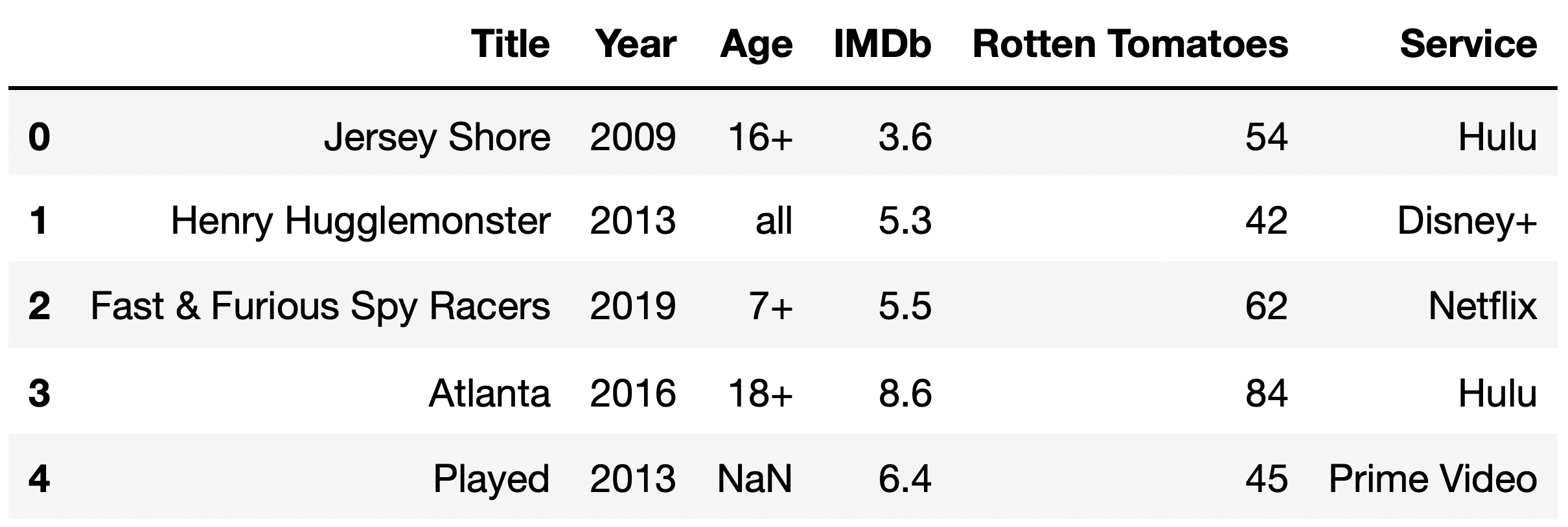
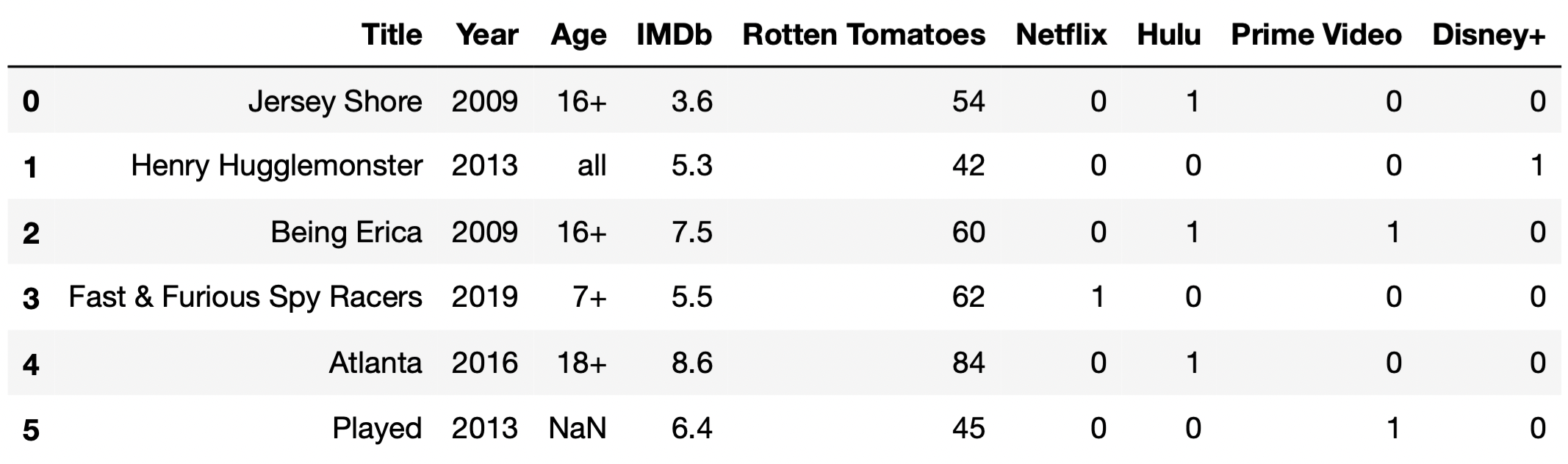
The DataFrame tv_excl contains all of the information we have for TV shows that are available to stream exclusively on a single streaming service. The "Service" column contains the name of the one streaming service that the TV show is available for streaming on.

The first few rows of tv_excl are shown below (though, of course, tv_excl has many more rows than are pictured here). Note that Being Erica is not in tv_excl, since it is available to stream on multiple services.

The DataFrame counts, shown in full below, contains the number of TV shows for every combination of "Age" and "Service".

Given the above information, what does the following expression evaluate to?

tv_excl.groupby(["Age", "Service"]).sum().shape[0]

• 4

• 5

• 12

• 16

• 18

• 20

• 25

Problem 11

The DataFrame flights contains information about recent flights, with each row representing a specific flight and the following columns:

• "flight num" (str): The unique code of the flight, consisting of a two-character airline designator followed by 1 to 4 digits (e.g., "UA1989").
• "airline" (str): The airline name (e.g., "United").
• "departure" (str): The code for the airport from which the flight departs (e.g., "SAN").
• "arrival" (str): The code for the airport at which the flight arrives (e.g., "LAX").

Suppose we have another DataFrame more_flights which contains the same columns as flights, but different rows. Define merged as follows.

        merged = flights.merge(more_flights, on = "airline")

Suppose that in merged, there are 108 flights where the airline is "United", and in more_flights, there are 12 flights where the airline is "United". If flights has 15 rows in total, how many of these rows are not for "United" flights? Give your answer as an integer.

Problem 12

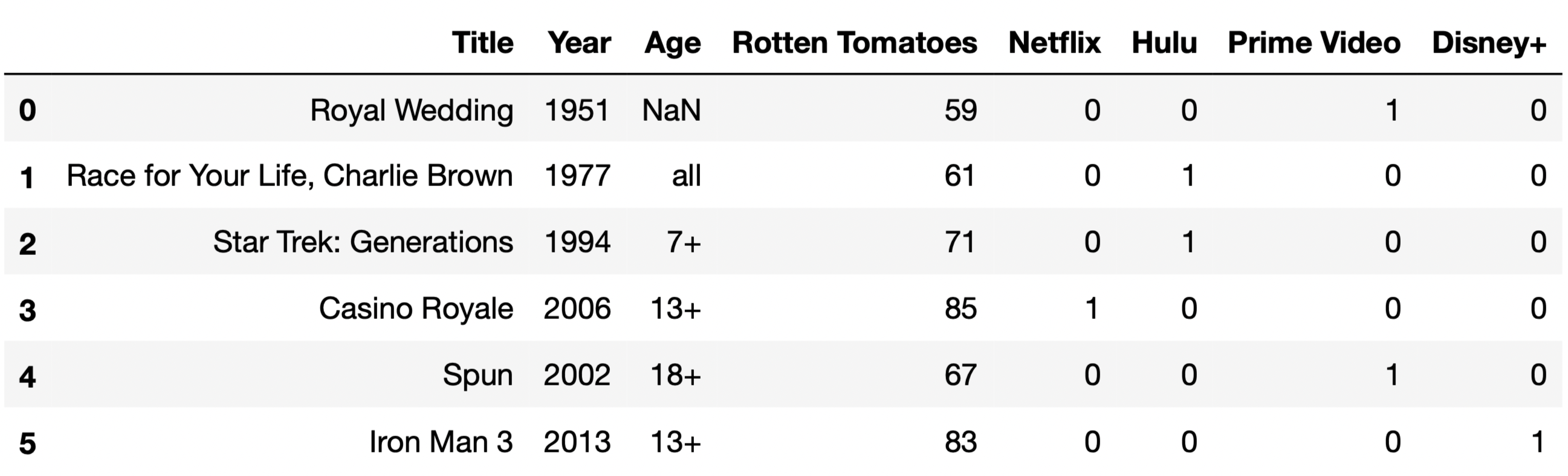
For your convenience, the first few rows of tv are shown again below.

For the purposes of this question only, suppose we have also access to another similar DataFrame, movies, which contains information about a variety of movies. The information we have for each movie in movies is the same as the information we have for each TV show in tv, except for IMDb ratings, which are missing from movies.

The first few rows of movies are shown below (though movies has many more rows than are pictured here).

Problem 12.1

The function total_null, defined below, takes in a DataFrame and returns the total number of null values in the DataFrame.

total_null = lambda df: df.isna().sum().sum()

Consider the function delta, defined below.

def delta(a, b):
    tv_a = tv.head(a)
    movies_b = movies.head(b)
    together = pd.concat([tv_a, movies_b])
    return total_null(together) - total_null(tv_a) - total_null(movies_b)

Which of the following functions is equivalent to delta?

• lambda a, b: a

• lambda a, b: b

• lambda a, b: 9 * a

• lambda a, b: 8 * b

• lambda a, b: min(9 * a, 8 * b)

Problem 12.2

Fill in the blank to complete the implementation of the function size_of_merge, which takes a string col, corresponding to the name of a single column that is shared between tv and movies, and returns the number of rows in the DataFrame tv.merge(movies, on=col).

• For instance, size_of_merge("Year") should return the number of rows in tv.merge(movies, on="Year").

• The purpose of this question is to have you think conceptually about how merges work. As such, solutions containing merge or concat will receive 0 points.

What goes in the blank below?

def size_of_merge(col):
    return (____).sum()

Hint: Consider the behavior below.

>>> s1 = pd.Series({'a': 2, 'b': 3})
>>> s2 = pd.Series({'c': 4, 'a': -1, 'b': 4})
>>> s1 * s2
a    -2.0
b    12.0
c     NaN
dtype: float64

Problem 13

For each day in May 2022, the DataFrame streams contains the number of streams for each of the “Top 200" songs on Spotify that day — that is, the number of streams for the 200 songs with the most streams on Spotify that day. The columns in streams are as follows:

• "date": the date the song was streamed

• "artist_names": name(s) of the artists who created the song

• "track_name": name of the song

• "streams": the number of times the song was streamed on Spotify that day

The first few rows of streams are shown below. Since there were 31 days in May and 200 songs per day, streams has 6200 rows in total.

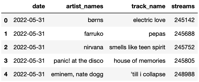
Note that:

• streams is already sorted in a very particular way — it is sorted by "date" in reverse chronological (decreasing) order, and, within each "date", by "streams" in increasing order.

• Many songs will appear multiple times in streams, because many songs were in the Top 200 on more than one day.

Problem 13.1

Complete the implementation of the function song_by_day, which takes in an integer day between 1 and 31 corresponding to a day in May, and an integer n, and returns the song that had the n-th most streams on day. For instance,
song_by_day(31, 199) should evaluate to "pepas", because "pepas" was the 199th most streamed song on May 31st.

Note: You are not allowed to sort within song_by_day — remember, streams is already sorted.

def song_by_day(day, n):
    day_str = f"2022-05-{str(day).zfill(2)}"
    day_only = streams[__(a)__].iloc[__(b)__]
    return __(c)__

What goes in each of the blanks?

Problem 13.2

Below, we define a DataFrame pivoted.

pivoted = streams.pivot_table(index="track_name", columns="date", 
                                values="streams", aggfunc=np.max)

After defining pivoted, we define a Series mystery below.

mystery = 31 - pivoted.apply(lambda s: s.isna().sum(), axis=1)

mystery.loc["pepas"] evaluates to 23. In one sentence, describe the relationship between the number 23 and the song "pepas" in the context of the streams dataset. For instance, a correctly formatted but incorrect answer is “I listened to the song "pepas" 23 times today."

Problem 13.3

In defining pivoted, we set the keyword argument aggfunc to np.max. Which of the following functions could we have used instead of np.max without changing the values in pivoted? Select all that apply.

• np.mean

• np.median

• len

• lambda df: df.iloc[0]

• None of the above

Problem 13.4

Below, we define another DataFrame another_mystery.

another_mystery = (streams.groupby("date").last()
                            .groupby(["artist_names", "track_name"])
                            .count().reset_index())

another_mystery has 5 rows. In one sentence, describe the significance of the number 5 in the context of the streams dataset. For instance, a correctly formatted but incorrect answer is “There are 5 unique artists in streams." Your answer should not include the word”row”.