from lec_utils import *
import lec20_util as util

Discussion Slides: Gradient Descent and Classification

Agenda 📆

• Gradient descent.
• Classification.
• Evaluating classification models.

Overview

• In order to find optimal model parameters, $w_0^*, w_1^*, ..., w_d^*$, our goal has been to minimize empirical risk.

$$R_\text{sq}(\vec w) = \frac{1}{n} \sum_{i = 1}^n (y_i - H(\vec x_i))^2$$Empirical risk using squared loss.

• We've minimized empirical risk functions (like $R$ above) a few ways so far:
  • Taking (partial) derivatives, setting them to 0, and solving.
  • Using a linear algebraic-argument, which led to the normal equations, $X^TX \vec w^* = X^T \vec y$.

• Gradient descent is a method for minimizing functions computationally, when doing so by hand is difficult or impossible.

Gradient descent

• Suppose we want to minimize a function $f$, which takes in a vector $\vec w$ as input and returns a scalar as output.
  For example, $f$ could be (but doesn't need to be) some empirical risk function, like the one on the previous slide.

• To do so:

  1. Start with an initial guess of the minimizing input, $\vec w^{(0)}$.
  2. Choose a learning rate, or step size, $\alpha$.
  3. Use the following update rule:

  $$\vec w^{(t+1)} = \vec w^{(t)} - \alpha \nabla f(\vec w^{(t)})$$

• $\nabla f(\vec{w}^{(t)})$ is the gradient of $f$, evaluated at timestep $t$.
  The gradient of a function is a vector containing all of its partial derivatives.

$$f(\vec{w}) = w_1^2 + w_2^2 \implies \nabla f(\vec w) = \begin{bmatrix} 2w_1 \\ 2w_2 \end{bmatrix}$$An example gradient calculation.

• We repeat this iterative process until convergence, i.e. until the changes between $\vec{w}^{(t+1)}$ and $\vec{w}^{(t)}$ are small (or equivalently, until $\nabla f(\vec w^{(t)})$ is close to $\vec 0$.

util.minimizing_animation(w0=0, alpha=0.01)

Regression vs. classification

• So far in the course, we've been working with regression problems – where our goal is to predict some quantitative variable.
  Examples: Predicting commute times, predicting house prices.

• With classification problems, our goal is to predict a categorical variable. These problems involve questions like:
  • Is this email spam or not? This is an example of binary classification, in which we predict one of two possible classes..
  • Is this picture of a dog, cat, zebra, or elephant? This is an example of multiclass classification, in which we predict one class from more than two possible options.

• We learned about two classification models in Wednesday's lecture: $k$-nearest neighbors and decision trees.

• The most common evaluation metric in classification is accuracy:

  $$\text{accuracy} = \frac{\text{# points classified correctly}}{\text{# points}}$$

  Accuracy ranges from 0 to 1, i.e. 0% to 100%. Higher values indicate better model performance.

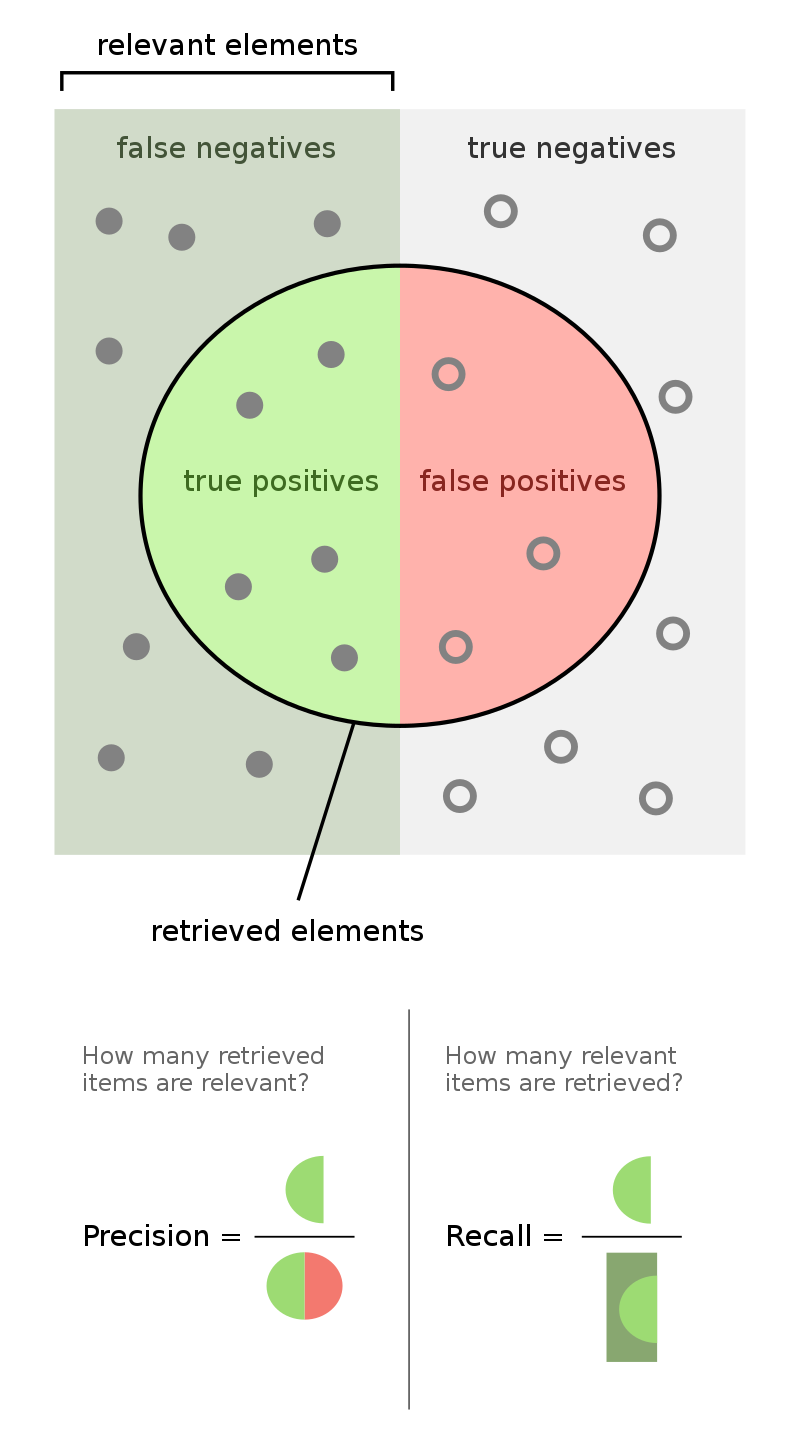
Evaluating classification models

• When we perform binary classification, there are 4 possible outcomes.

Outcome of Prediction	Definition	True Class
True positive (TP) ✅	The predictor correctly predicts the positive class.	P
False negative (FN) ❌	The predictor incorrectly predicts the negative class.	P
True negative (TN) ✅	The predictor correctly predicts the negative class.	N
False positive (FP) ❌	The predictor incorrectly predicts the positive class.	N

• We often evaluate classifiers using precision and recall.

$$\text{precision} = \frac{TP}{TP + FP} \: \: \: \: \: \: \: \: \text{recall} = \frac{TP}{TP + FN}$$