from lec_utils import *

Discussion Slides: Feature Engineering and Pipelines

Agenda 📆

• Feature engineering.
• Pipelines.
• One hot encoding.

Feature engineering

• Feature engineering is the act of finding transformations that transform data into effective quantitative variables.
  Put simply: feature engineering is creating new features using existing features. Our model can then fit different weights for each new feature we create.

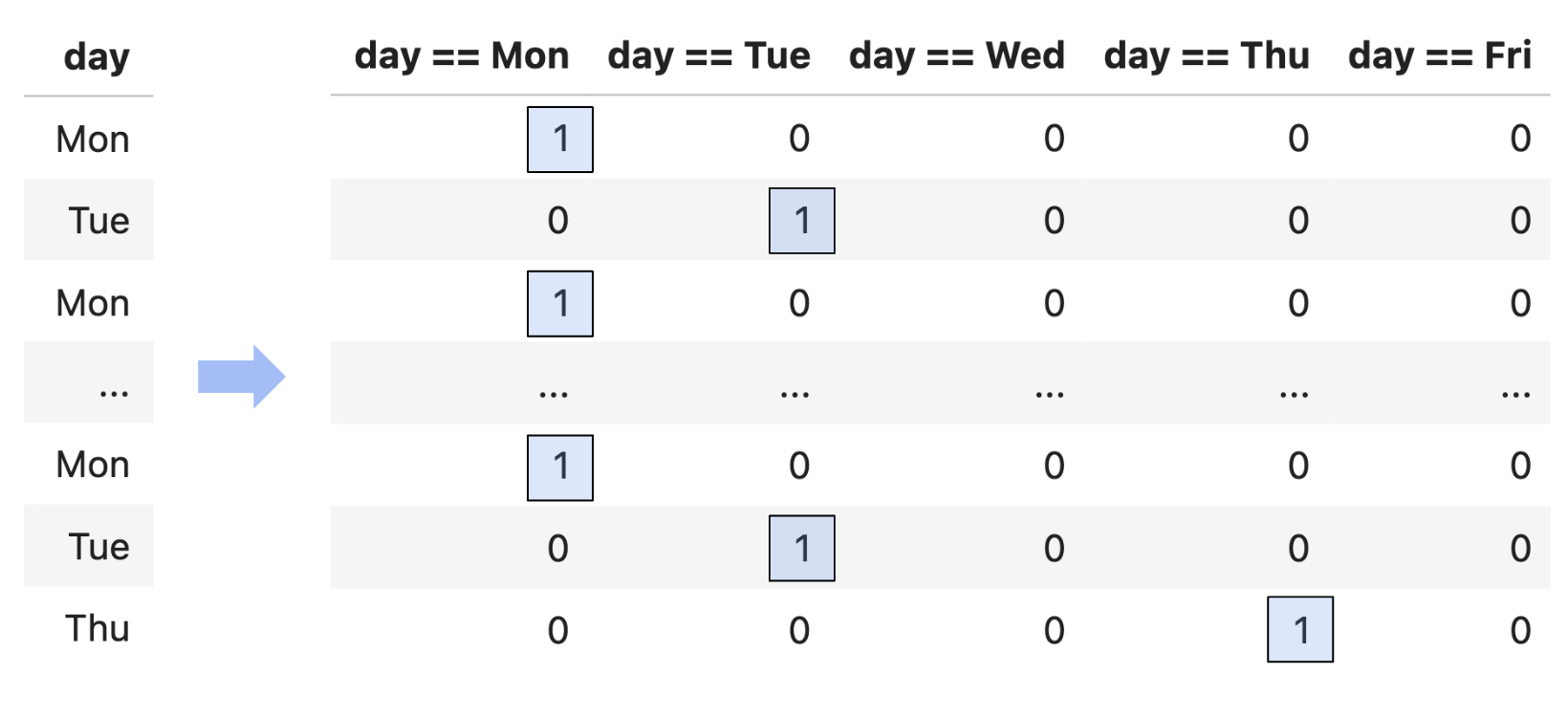
• Example: One hot encoding, in which we transform one column of categorical variables into several binary features.

Transformation Type	Purpose	Example	sklearn Syntax
One-Hot Encoding	Converts a categorical variable with $N$ unique values into $N-1$ binary features. Each indicator is 1 if the observation is in that category (with one dropped as the baseline).	Before: conference = ["ACC", "SEC", "Big Ten"] After: conference_SEC = [0, 1, 0], conference_Big Ten = [0, 0, 1] We drop one column ("ACC") when one-hot encoding.	OneHotEncoder(drop='first')
Polynomial Features	Expands a numerical variable by adding higher-order terms to capture non-linear relationships.	Before: seed = [1, 4, 2] After: seed = [1, 4, 2], seed^2 = [1, 16, 4], seed^3 = [1, 64, 8]	PolynomialFeatures(degree=3, include_bias=False)
Standardization	Rescales features so that they have a mean of 0 and a standard deviation of 1, making them directly comparable.	Before: seed = [1, 3, 2] After: seed_std ≈ [-1.225, 1.225, 0]	StandardScaler()
Function Transformation	Applies a custom function to a feature, e.g., to bin continuous values into categories.	Before: day_of_month = [5, 16, 22, 30] After: day_bin = ["early", "late", "late", "late"] We would then one-hot encode this feature.	FunctionTransformer(lambda X: np.where(X <= 15, "early", "late").reshape(-1, 1))

Use this as a reference; don't try and memorize it.

Pipelines

• A Pipeline in sklearn is a way to chain multiple feature engineering and model building steps together.

• For example, let's build a Pipeline that predicts a team's March Madness 'tournament_wins'.
  You'll do something similar in Homework 8, which will be released soon.

df = pd.DataFrame({
    "seed": [1, 4, 2, 8, 3, 12],
    "conference": ["ACC", "Big Ten", "ACC", "SEC", "Big Ten", "American"],
    "win_percentage": [0.90, 0.75, 0.88, 0.65, 0.80, 0.9],
    "tournament_wins": [6, 3, 5, 1, 4, 1]
})
df

	seed	conference	win_percentage	tournament_wins
0	1	ACC	0.90	6
1	4	Big Ten	0.75	3
2	2	ACC	0.88	5
3	8	SEC	0.65	1
4	3	Big Ten	0.80	4
5	12	American	0.90	1

• Specifically, we'll:
  • One hot encode a team's 'conference'.
  • Create polynomial features out of the 'seed' column.
  
  Why might we want to add a polynomial feature to a seemingly linear column ('seed')? Although seed values are integers representing rankings (with smaller numbers indicating better-ranked teams), their relationship with tournament wins may not be strictly linear. For instance, the jump in performance from a 1 seed to a 2 seed might be different from the jump from a 7 seed to an 8 seed. A polynomial transformation could help us capture this.

Constructing our Pipeline

• A Pipeline is made up of one or more transformers, followed (optionally) by an estimator.
  Transformers, as we saw in the table a few slides ago, are used for creating features. Estimators are model objects, like LinearRegression.

• To create a Pipeline, either use the Pipeline constructor or the make_pipeline function.
  Eventually, we will create our final Pipeline as follows:

  model = make_pipeline(
      SomeTransformer, # Doesn't exist yet!
      LinearRegression()
  )
  
  model.fit(X=df[['seed', 'conference', 'win_percentage']], y=df['tournament_wins'])
  

from sklearn.pipeline import Pipeline, make_pipeline

• To tell sklearn to perform different transformations on different columns, create a ColumnTransformer object.

from sklearn.compose import ColumnTransformer, make_column_transformer
from sklearn.preprocessing import PolynomialFeatures, OneHotEncoder, FunctionTransformer

# Here, we one-hot encode the 'conference' column and drop the first category to avoid multicollinearity (which we'll talk about soon!)
SomeTransformer = make_column_transformer(
    (OneHotEncoder(drop='first'), ['conference']),
    (PolynomialFeatures(degree=3, include_bias=False), ['seed']),
    remainder='passthrough' # The remaining feature, 'win_percentage', is kept unchanged (the alternative is remainder='drop').
)
SomeTransformer

ColumnTransformer(remainder='passthrough',
                  transformers=[('onehotencoder', OneHotEncoder(drop='first'),
                                 ['conference']),
                                ('polynomialfeatures',
                                 PolynomialFeatures(degree=3,
                                                    include_bias=False),
                                 ['seed'])])

In a Jupyter environment, please rerun this cell to show the HTML representation or trust the notebook.
On GitHub, the HTML representation is unable to render, please try loading this page with nbviewer.org.

• Now, we're ready to build our actual Pipeline.

from sklearn.linear_model import LinearRegression

model = make_pipeline(
    SomeTransformer,
    LinearRegression()
)

model.fit(X=df[['seed', 'conference', 'win_percentage']], y=df['tournament_wins'])

Pipeline(steps=[('columntransformer',
                 ColumnTransformer(remainder='passthrough',
                                   transformers=[('onehotencoder',
                                                  OneHotEncoder(drop='first'),
                                                  ['conference']),
                                                 ('polynomialfeatures',
                                                  PolynomialFeatures(degree=3,
                                                                     include_bias=False),
                                                  ['seed'])])),
                ('linearregression', LinearRegression())])

In a Jupyter environment, please rerun this cell to show the HTML representation or trust the notebook.
On GitHub, the HTML representation is unable to render, please try loading this page with nbviewer.org.

Using our Pipeline

• After fitting, we can print our model's optimal parameters and transformed features!

model

Pipeline(steps=[('columntransformer',
                 ColumnTransformer(remainder='passthrough',
                                   transformers=[('onehotencoder',
                                                  OneHotEncoder(drop='first'),
                                                  ['conference']),
                                                 ('polynomialfeatures',
                                                  PolynomialFeatures(degree=3,
                                                                     include_bias=False),
                                                  ['seed'])])),
                ('linearregression', LinearRegression())])

In a Jupyter environment, please rerun this cell to show the HTML representation or trust the notebook.
On GitHub, the HTML representation is unable to render, please try loading this page with nbviewer.org.

model.named_steps # Useful to see what each individual step is named; these names are chosen automatically by the helper functions.

{'columntransformer': ColumnTransformer(remainder='passthrough',
                   transformers=[('onehotencoder', OneHotEncoder(drop='first'),
                                  ['conference']),
                                 ('polynomialfeatures',
                                  PolynomialFeatures(degree=3,
                                                     include_bias=False),
                                  ['seed'])]),
 'linearregression': LinearRegression()}

model[-1]

LinearRegression()

In a Jupyter environment, please rerun this cell to show the HTML representation or trust the notebook.
On GitHub, the HTML representation is unable to render, please try loading this page with nbviewer.org.

print("Intercept:", model.named_steps['linearregression'].intercept_)
feature_names = model.named_steps['columntransformer'].get_feature_names_out()

# Print each feature with its corresponding coefficient.
for name, coef in zip(feature_names, model.named_steps['linearregression'].coef_):
    print(f"{name}: {coef}")

Intercept: 6.934953151584841
onehotencoder__conference_American: -0.17628833874649633
onehotencoder__conference_Big Ten: 0.022351765334817735
onehotencoder__conference_SEC: 0.8995467516086498
polynomialfeatures__seed: -0.8839029113326689
polynomialfeatures__seed^2: -0.05619241815616135
polynomialfeatures__seed^3: 0.007489714047328858
remainder__win_percentage: -0.0026083734926004684

• Thus, our hypothesis function looks like:

  $$ \text{pred. number of games won}_i = 6.935 - 0.176\cdot \{\text{conference}_i == \text{American}\} + 0.022\cdot \{\text{conference}_i == \text{Big Ten}\} + 0.900\cdot \{\text{conference}_i == \text{SEC}\} - 0.884\cdot \text{seed}_i - 0.056\cdot \text{seed}_i^2 + 0.007\cdot \text{seed}_i^3 - 0.003\cdot \text{win percentage}_i $$

  Notice how we don't have a one hot encoded parameter for the ACC 'conference', since we used drop='first' in our OneHotEncoder.

• Once our pipeline is fit, we can use it to make predictions.
  For example, what's the predicted number of tournament wins for Michigan this year?

michigan = pd.DataFrame({
    'seed': [5],
    'conference': ['Big Ten'],
    'win_percentage': [0.735],
})

predicted_wins = model.predict(michigan)
print("Predicted Tournament Wins:", predicted_wins[0])

Predicted Tournament Wins: 2.0672770077513265

Why do we drop one column when one hot encoding?

• Consider what our design matrix, $X$, would look like if we don't drop the one hot encoded ACC column.

$$ X = \left[ \begin{array}{ccccccccc} % Data rows: 1 & 1 & 1 & 1 & 1 & 0 & 0 & 0 & 0.90 \\ 1 & 4 & 16 & 64 & 0 & 1 & 0 & 0 & 0.75 \\ 1 & 2 & 4 & 8 & 1 & 0 & 0 & 0 & 0.88 \\ 1 & 8 & 64 & 512 & 0 & 0 & 1 & 0 & 0.65 \\ 1 & 3 & 9 & 27 & 0 & 1 & 0 & 0 & 0.80 \\ 1 & 12 & 144 & 1728 & 0 & 0 & 0 & 1 & 0.90 \\ % Spacing before label row: % Label row (must match the same 9 columns): \underbrace{\phantom{1}}_{\text{intercept}} & \underbrace{\phantom{1}}_{\text{seed}} & \underbrace{\phantom{1}}_{\text{seed}^2} & \underbrace{\phantom{1}}_{\text{seed}^3} & \underbrace{\phantom{1}}_{\text{ACC}} & \underbrace{\phantom{1}}_{\text{Big Ten}} & \underbrace{\phantom{1}}_{\text{SEC}} & \underbrace{\phantom{1}}_{\text{American}} & \underbrace{\phantom{0.90}}_{\text{win percentage}} \end{array} \right] $$

• Notice that we can write our intercept column, $\vec{1}$ as a linear combination of our one hot encoded columns:

  $$\vec{1} = \vec{\text{ACC}} + \vec{\text{Big Ten}} + \vec{\text{SEC}} + \vec{\text{American}}$$

  This means there is multicollinearity present: one of our features is redundant.

• The columns of $X$ are not linearly independent, so:

  • $X$ is not full rank, so
  • $X^TX$ is not full rank, so
  • $X^TX$ isn't invertible, so
  • there are infinitely many solutions to the normal equations,

  $$X^TX \vec w = X^T \vec y$$

Avoiding multicollinearity

• When there is multicollinearity present, we don't know which of the infinitely many solutions sklearn will give back to us. The resulting coefficients of the fit model are uninterpretable.

$$ \text{pred. number of games won}_i = \boxed{1.5} + \boxed{2} \cdot \{\text{conference}_i == \text{ACC}\} + \boxed{1} \cdot \{\text{conference}_i == \text{Big Ten}\} + \boxed{4} \cdot \{\text{conference}_i == \text{SEC}\} + \boxed{0.5} \cdot \{\text{conference}_i == \text{American}\} $$ $$ \text{pred. number of games won}_i = \boxed{100} - \boxed{96.5} \cdot \{\text{conference}_i == \text{ACC}\} - \boxed{97.5} \cdot \{\text{conference}_i == \text{Big Ten}\} - \boxed{94.5} \cdot \{\text{conference}_i == \text{SEC}\} - \boxed{98} \cdot \{\text{conference}_i == \text{American}\} $$

• To avoid multicollinearity and guarantee a unique solution for our optimal parameters, we drop one of the one hot encoded columns (typically using OneHotEncoder(drop='first')).

• Remember, multicollinearity doesn't impact a model's predictions!