from lec_utils import *

Discussion Slides: Loss Functions and Simple Linear Regression

Agenda 📆

• The modeling recipe 👨‍🍳.
• Loss vs. empirical risk.
• Worksheet 📝.

What are models?

• A model is a set of assumptions about how data was generated.

• When a model fits the data well, it can provide a useful approximation to the world or simply a helpful description of the data.

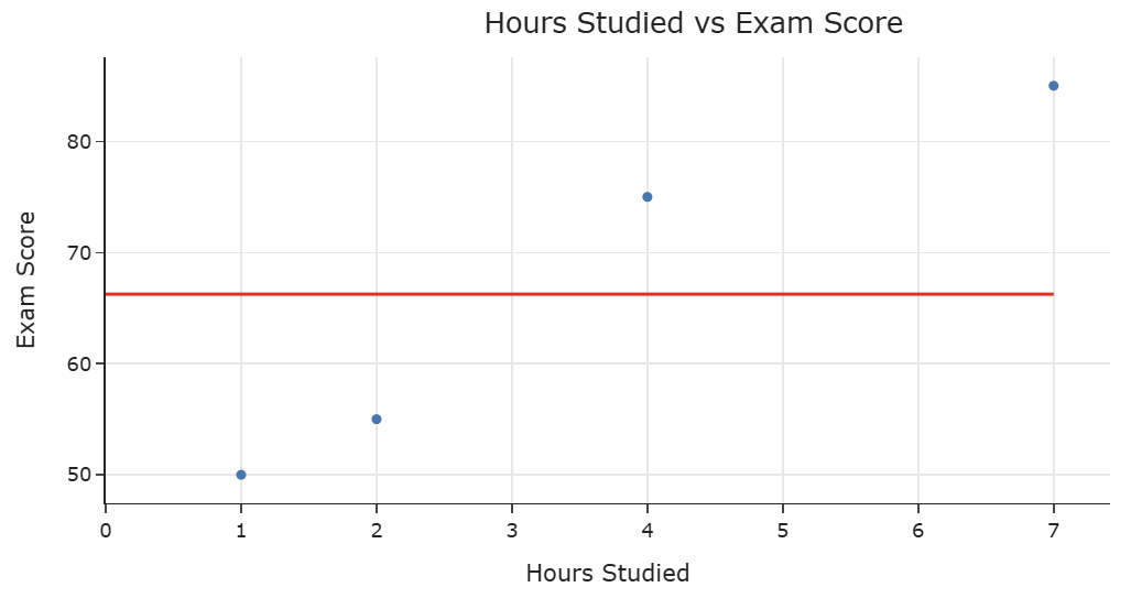For example, this is the constant model, which picks a constant output regardless of the input.

• Million dollar question: Suppose we choose to build a constant model. Of all possible constant predictions for a particular dataset, which constant prediction do we choose?

What is loss?

• A loss function measures how "off" our model's predictions are for a single prediction. If our prediction is totally off, the loss function will output a higher number, whereas if it's good, it will output a lower number.

• One common loss function is the squared loss function, which measures the squared error between the true value $y_i$ and our predicted value $H(x_i)$.

$$ L_\text{sq}(y_i, H(x_i)) = (y_i - H(x_i))^2 $$

• For example, if our model estimated a y-value of $10$ on an input of $x = 5$, but the true y-value in our data was $15$ when $x = 5$, then our squared loss function would output $(15-10)^2 = 25$.

Empirical risk

• Let's consider again the constant model, where our predictions are a fixed value, $h$, that does not depend on the input ($x_i$). That is, we define our model as:

$$ H(x_i) = h $$

• For a dataset with $n$ data points ${(x_1, y_1), (x_2, y_2), \dots, (x_n, y_n)}$, the squared loss for each point is:

$$ L_\text{sq}(y_i, H(x_i)) = (y_i - h)^2 $$

• The empirical risk function, $R$, averages the loss function to across the entire dataset, providing a measure of how accurately our prediction model performs across all data points.

• In the case of the constant model with squared loss, the empirical risk looks like:

$$ R_{\text{sq}}(h) = \frac{1}{n} \sum_{i=1}^{n} (y_i - h)^2 = (y_1 - h)^2 + (y_2 - h)^2 + ... + (y_n - h)^2 $$There are lots of names for $R_\text{sq}$: average squared loss, mean squared error, empirical risk

• The optimal model parameters are the ones that minimize empirical risk!

• In lecture, we showed that $h^* = \text{Mean}(y_1, y_2, ..., y_n)$ minimizes $R_\text{sq}(h)$.
  That means the best constant prediction when using squared loss is the mean of the data.

Loss vs. empirical risk

• Loss measures the quality of a single prediction made by a model.

$$L_\text{sq}(y_i, h) = (y_i - h)^2$$

• Empirical risk measures the average quality of all predictions made by a model.

$$R_\text{sq}(h) = \frac{1}{n} \sum_{i=1}^n (y_i - h)^2$$

• To find optimal model parameters, we minimize empirical risk!

The modeling recipe

1. Choose a model.
   • Example: Constant model, $H(x_i) = h$.
   • Example: Simple linear regression model, $H(x_i) = w_0 + w_1 x_i$.

2. Choose a loss function.
   • Example: Squared loss, $L_\text{sq}(y_i, H(x_i)) = (y_i - H(x_i))^2$.
   • Example: Absolute loss, $L_\text{abs}(y_i, H(x_i)) = | y_i - H(x_i) |$.

3. Minimize average loss to find optimal model parameters.
   • Constant model + squared loss: $h^* = \text{Mean}(y_1, y_2, ..., y_n)$.
   • Constant model + absolute loss: $h^* = \text{Median}(y_1, y_2, ..., y_n)$.
   • Simple linear regression model + squared loss: $w_1^* = r \frac{\sigma_y}{\sigma_x}, w_0^* = \bar{y} - w_1^* \bar{x}$.