from lec_utils import *

Discussion Slides: Grouping, Pivoting, and Merging

Agenda 📆

• The groupby method.
• Pivot tables.
• merge and types of merges.
• Worksheet 📝.

Today's Dataset 🏈〽️

• Today, we're going to be working with a dataset on the past 100 years of Michigan Football.
  Source: www.mgoblue.com.

• Like last week, let's store our dataset in the df variable.

df = pd.read_csv('data/michigan_football.csv')
df

	year	opponent	venue	result	UM_score	opp_score	date	time
0	2024	Fresno State	Home	W	30.0	10.0	Aug 31 (Sat)	7:30 PM
1	2024	#3 Texas	Home	L	12.0	31.0	Sep 7 (Sat)	Noon
2	2024	Arkansas State	Home	W	28.0	18.0	Sep 14 (Sat)	Noon
...	...	...	...	...	...	...	...	...
1100	1924	Northwestern	Home	W	27.0	0.0	Nov 8 (Sat)	NaN
1101	1924	Ohio State	Away	W	16.0	6.0	Nov 15 (Sat)	NaN
1102	1924	Iowa (HC)	Home	L	2.0	9.0	Nov 22 (Sat)	NaN

1103 rows × 8 columns

df.columns

Index(['year', 'opponent', 'venue', 'result', 'UM_score', 'opp_score', 'date',
       'time'],
      dtype='object')

Read the DataFrame internals guide!

• We've posted a guide, DataFrame Internals, that you should read.

• It covers various topics, like:

  • How to add columns to DataFrames without side effects.
  • How to write functions that manipulate DataFrames without side effects.
  • How to use Series methods, like mean and describe, on DataFrames.
  
  

  and more!

The groupby method

• Key idea: If the information we want involves performing some operation separately for each group, we use groupby.

• For instance, if we want to find the average number of points Michigan scored each year, we use groupby('year').

df.groupby('year')['UM_score'].mean()

year
1924    19.38
1925    28.38
1926    23.88
        ...  
2022    40.43
2023    35.87
2024    22.00
Name: UM_score, Length: 101, dtype: float64

• df.groupby('year')['UM_score'].mean()
  First, we need to tell pandas which column we want to group by. Since we're grouping by 'year', the remainder of the calculations will be done separately for each 'year'.

• df.groupby('year')['UM_score'].mean()
  Then, select the other column(s) that you want to aggregate. Here, we want to calculate the mean 'UM Score', so that's what we select.

• df.groupby('year')['UM_score'].mean()
  Finally, we use an aggregation method. This is saying, for each 'year', compute the mean 'UM Score'.

Reference Slide

The split, apply, combine process

• Under the hood, groupby follows 3 steps: split, apply, and combine.

• We start by splitting rows into distinct groups.
  When we use df.groupby('year'), the groups are created by separating rows based on 'year' values.

# The 2024 group and 2023 group.
# df.groupby('year') will create separate groups for each 'year.'
group_2024 = df.loc[df['year'] == 2024]
group_2023 = df.loc[df['year'] == 2023]
dfs_side_by_side(group_2024.head(), group_2023.head())

	year	opponent	venue	result	UM_score	opp_score	date	time
0	2024	Fresno State	Home	W	30.0	10.0	Aug 31 (Sat)	7:30 PM
1	2024	#3 Texas	Home	L	12.0	31.0	Sep 7 (Sat)	Noon
2	2024	Arkansas State	Home	W	28.0	18.0	Sep 14 (Sat)	Noon
3	2024	#11 USC	Home	W	27.0	24.0	Sep 21 (Sat)	3:30 PM
4	2024	Minnesota	Home	W	27.0	24.0	Sep 28 (Sat)	Noon

	year	opponent	venue	result	UM_score	opp_score	date	time
13	2023	East Carolina	Home	W	30.0	3.0	Sep 2 (Sat)	Noon
14	2023	UNLV	Home	W	35.0	7.0	Sep 9 (Sat)	3:30 PM
15	2023	Bowling Green	Home	W	31.0	6.0	Sep 16 (Sat)	7:30 PM
16	2023	Rutgers	Home	W	31.0	7.0	Sep 23 (Sat)	12:00 PM
17	2023	Nebraska	Away	W	45.0	7.0	Sep 30 (Sat)	2:30 PM CT

• Then, we apply the operation to each group, individually.

print("2024 result:", group_2024['UM_score'].mean())
print("2023 result:", group_2023['UM_score'].mean())
print("and so on...")

2024 result: 22.0
2023 result: 35.86666666666667
and so on...

• Finally, we combine the results of the operation on each group into a single Series or DataFrame (depending on the operation).

df.groupby('year')['UM_score'].mean().sort_index(ascending=False)

year
2024    22.00
2023    35.87
2022    40.43
        ...  
1926    23.88
1925    28.38
1924    19.38
Name: UM_score, Length: 101, dtype: float64

• In the expression below, mean is an aggregation method.
  It takes many 'UM_score' values for a particular 'year' and combines them into a single value.

Reference Slide

Aggregating

df.groupby('year')['UM_score'].mean()

year
1924    19.38
1925    28.38
1926    23.88
        ...  
2022    40.43
2023    35.87
2024    22.00
Name: UM_score, Length: 101, dtype: float64

• Sometimes, we want to perform:
  • An aggregation that doesn't have a built-in implementation.
  • Different aggregation methods on different columns.

• The aggregate method, or agg for short, is the general-purpose tool for performing aggregations.

# Finds the average score, and the win percentage, for home vs. away games.
(
    df
    .groupby('venue')
    .agg({
        'UM_score': 'mean', # equivalent to df.groupby('venue')['UM_score'].mean()
        # the parameter `s` here is a Series of the 'result' values for each group.
        'result': lambda s: (s == 'W').sum() / len(s) 
    })
)

	UM_score	result
venue
Away	23.59	0.65
Home	27.35	0.74

• 📢 Michigan performs significantly better at home, both in terms of points scored and win percentage!

Filtering

• So far, the only operations we've applied to each group is some sort of aggregation (i.e. aggregating the mean score across years).

• Instead of aggregating, perhaps we want to only keep groups that satisfy a certain condition.
  To do so, we use the filter method instead of any aggregation method.

• For instance, if we want to keep only the 'year's in which Michigan won at least 12 games:

def has_at_least_twelve_wins(group):
    # has_at_least_twelve_wins is called separately for each 'year'.
    # Each time it's called, the `group` argument is a DataFrame.
    return (group['result'] == 'W').sum() >= 12

twelveplus_wins = df.groupby('year').filter(has_at_least_twelve_wins)
twelveplus_wins

	year	opponent	venue	result	UM_score	opp_score	date	time
13	2023	East Carolina	Home	W	30.0	3.0	Sep 2 (Sat)	Noon
14	2023	UNLV	Home	W	35.0	7.0	Sep 9 (Sat)	3:30 PM
15	2023	Bowling Green	Home	W	31.0	6.0	Sep 16 (Sat)	7:30 PM
...	...	...	...	...	...	...	...	...
367	1997	#23 Wisconsin	Away	W	26.0	16.0	Nov 15 (Sat)	2:30 PM CT
368	1997	#4 Ohio State	Home	W	20.0	14.0	Nov 22 (Sat)	Noon
369	1997	#8 Washington State	NaN	W	21.0	16.0	Jan 1 (Thu)	2:00 PM PT

58 rows × 8 columns

twelveplus_wins['year'].unique()

array([2023, 2022, 2021, 1997])

Pivot tables

• It's possible to use groupby on two columns at once, e.g. df.groupby(['year', 'venue']).
  The resulting operations are performed separately for every unique combination of values in the specified columns.
  See Lecture 5 for examples. We can also group on three or more columns too!

# The index here is a MultiIndex.
df.groupby(['year', 'venue'])['UM_score'].mean()

year  venue
1924  Away     12.50
      Home     26.25
1925  Away     12.00
               ...  
2023  Home     35.71
2024  Away     13.00
      Home     26.88
Name: UM_score, Length: 202, dtype: float64

• Rather than grouping on two columns at once, we can create a pivot table, which also shows the result of aggregating by two columns at once but in a more human-readable way.

df.pivot_table(index='year', columns='venue', values='UM_score', aggfunc='mean')

venue	Away	Home
year
1924	12.50	26.25
1925	12.00	40.20
1926	12.00	33.40
...	...	...
2022	38.75	40.38
2023	40.20	35.71
2024	13.00	26.88

101 rows × 2 columns

• The DataFrame above has:
  • One row for every unique value in index.
  • One column for every unique value in columns.
  • Values determined by applying aggfunc on values in values.

• Notice how the value 12.50 at (1924, 'Away') in our MultiIndex groupby result matches the corresponding value in our pivot table! Michigan scored 12.5 points away on average in 1924.

Merging

• We merge DataFrames when we have two sources of information about the same individuals that is linked by a common column(s).
  The common column(s) are called the join key.
  In SQL, we call this operation a JOIN.

• When we merge DataFrames, we have to specify how to merge the DataFrames, in the (likely) event that there are rows in the two DataFrames that don't match.

• To help us visualize these operations, we'll redefine df to be a smaller subset of our original DataFrame.

# Smaller game DataFrame
df = pd.DataFrame({
    "year": [2024, 2024, 2023, 2023, 2022],
    "opponent": ["Washington", "Alabama", "Washington", "Michigan State", "Oregon"],
    "venue": ["Home", "Away", "Away", "Home", "Home"],
    "result": ["L", "W", "L", "W", "L"]
})

# Big Ten Teams DataFrame (5 rows)
big_10 = pd.DataFrame({
    "team": ["Minnesota", "Michigan State", "Washington", "Ohio State", "Oregon"],
    "coach": ["P.J. Fleck", "Mel Tucker", "Kalen DeBoer", "Ryan Day", "Dan Lanning"],
    "location": ["Minneapolis, MN", "East Lansing, MI", "Seattle, WA", "Columbus, OH", "Eugene, OR"]
})

dfs_side_by_side(df, big_10)

	year	opponent	venue	result
0	2024	Washington	Home	L
1	2024	Alabama	Away	W
2	2023	Washington	Away	L
3	2023	Michigan State	Home	W
4	2022	Oregon	Home	L

	team	coach	location
0	Minnesota	P.J. Fleck	Minneapolis, MN
1	Michigan State	Mel Tucker	East Lansing, MI
2	Washington	Kalen DeBoer	Seattle, WA
3	Ohio State	Ryan Day	Columbus, OH
4	Oregon	Dan Lanning	Eugene, OR

• An inner merge keeps only the rows where the keys match in both DataFrames. In this case, it keeps the games where Michigan played teams from the Big 10 (based on the opponent column in df and the team column in big_10). Notice how the resulting DataFrame includes all columns from both DataFrames, but only for rows where there’s a match."

df.merge(big_10, left_on="opponent", right_on="team", how="inner")

	year	opponent	venue	result	team	coach	location
0	2024	Washington	Home	L	Washington	Kalen DeBoer	Seattle, WA
1	2023	Washington	Away	L	Washington	Kalen DeBoer	Seattle, WA
2	2023	Michigan State	Home	W	Michigan State	Mel Tucker	East Lansing, MI
3	2022	Oregon	Home	L	Oregon	Dan Lanning	Eugene, OR

Merging Activity

Activity

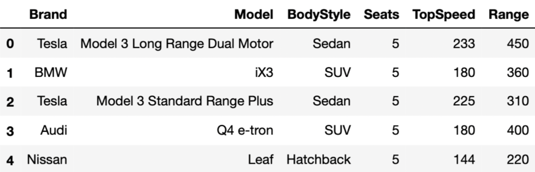
Consider the following DataFrame, evs, which has 32 rows total.

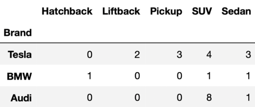
And consider the pivot table that contains the distribution of “BodyStyle” for all “Brands” in evs, other than Nissan.

evs.pivot_table(index='Brand', columns='BodyStyle', values='BodyStyle', aggfunc='count').

Suppose we ran the following lines of code:

tesla = evs[evs.get("Brand") == "Tesla"]

bmw = evs[evs.get("Brand") == "BMW"]

audi = evs[evs.get("Brand") == "Audi"]

Question: How many rows does the DataFrame combo have?

combo = tesla.merge(bmw, on="BodyStyle").merge(audi, on="BodyStyle")

Hint: When we leave the how parameter empty, .merge defaults to an inner join.

Click here to see the answer to the previous activity.

Answer: 35

First, we need to determine the number of rows in tesla.merge(bmw, on="BodyStyle"), and then determine the number of rows in combo. For the purposes of the solution, let’s use temp to refer to the first merged DataFrame, tesla.merge(bmw, on="BodyStyle").

Step 1: Merging Tesla and BMW (temp)

When merging two DataFrames, the resulting DataFrame (temp) contains a row for every match between the two columns being merged, while rows without matches are excluded. In this case, the column of interest is BodyStyle.

Matches Between Tesla and BMW:

• SUV: Tesla has $4$ rows for "SUV", and BMW has $1$ row for "SUV".
  $$ 4 \times 1 = 4 \text{ SUV rows in } temp $$
  
• Sedan: Tesla has $3$ rows for "Sedan", and BMW has $1$ row for "Sedan".
  $$ 3 \times 1 = 3 \text{ Sedan rows in } temp $$
  

Thus, the total number of rows in temp is: $$ 4 + 3 = 7 \text{ rows} $$

Step 2: Merging temp with Audi (combo)

Now, we merge temp with the Audi DataFrame, again on BodyStyle. Each row in temp matches with rows in Audi based on the same "BodyStyle".

Matches Between temp and Audi:

• SUV: temp has $4$ rows for "SUV", and Audi has $8$ rows for "SUV".
  $$ 4 \times 8 = 32 \text{ SUV rows in } combo $$
  
• Sedan: temp has $3$ rows for "Sedan", and Audi has $1$ row for "Sedan".
  $$ 3 \times 1 = 3 \text{ Sedan rows in } combo $$
  

Thus, the total number of rows in combo is: $$ 32 + 3 = 35 $$

Note: You may notice that 35 is the result of multiplying the "SUV" and "Sedan" columns in the DataFrame provided, and adding up the results.